← Modules

DynamicalSystem

The DynamicalSystem class is the foundational abstraction in pykal for modeling any control-system component (plant, controller, observer, sensor, estimator, etc.). This notebook demonstrates the core usage patterns of DynamicalSystem through progressively more complex examples. But first, the “Conceptual Foundation” section will cover the mathematical and programmatic foundation behind the DynamicalSystem class. Do not skip this section; reading it will solve a hundred problems before they start!

Conceptual Foundation

We begin with the minimal mathematics needed to define the discrete-time dynamical systems. We then introduce notational conventions and end with a Python implementation of the concepts discussed.

Discrete-Time Dynamical Systems

Note

This is a minimal category-theoretic definition of the discrete-time dynamical system. For an intuitive overview, including how to case continous-time dynamical systems as discrete-time dynamical systems, check out Steve Brunton’s video. For a reference to the category theoretic concepts needed here (which are quite minimal), check out the relevant wikipedia article on the category \(\text{Set}\).

Consider the category \(\text{Set}\). Let \(T \in \text{Set}\) where \(T \subset \mathbb{R}^+ \) and \(T\) has finite cardinality \(|T| = N\). We will refer to such a set as a time domain. Given a time domain \(T\), we may construct an indexing set \(K=\left\{ 1,2,\dots,N\right\}\), where \( k \in K\) indexes elements of our time domain \(T\) as \(t_k\). In so doing, \(T\) becomes an indexed time domain.

Now let \(X, Y, \mathcal{M} \in \text{Set}\). We will refer to \(X\) as the state space, \(Y\) as the output space, and \(\mathcal{M}\) the parameter space. We place the following restriction on our choice of \(X,Y\), and \(\mathcal{M}\):

• No space in the triple \((X,Y,\mathcal{M})\) is empty.

• At least one space in the triple \((X,Y,\mathcal{M})\) must have \(|T| = N\) elements.

We will now construct a special function that will map a subset of \(X \times \mathcal{M}\) with a subset of \(X \times Y\). We will call such a function a discrete-time dynamical system.

First, consider the product \(X \times \mathcal{M} \times X \times Y\). Such a product will clearly have cardinality \(|X| \cdot |\mathcal{M}| \cdot |X| \cdot |Y| \geq N\) (by the restriction above); thus, we may arbitrarily index a subset of the product \(X \times \mathcal{M} \times X \times Y\) using the indexing set \(K-1:=\left\{ 1,2,\dots,N-1\right\}\) with indices \(k\) as follows:

\[ (x_k,\mu_k,x_{k+1},y_j) \in X \times \mathcal{M} \times X \times Y. \]

We may split each tuple \((x_k,\mu_k,x_{k+1},y_k)\) into a tuple of tuples \(((x_k,\mu_k),(x_{k+1},y_j))\), where, by the ordered pair definition of a function, we have created a map

\[ (x_k,\mu_k) \mapsto (x_{k+1},y_k) \]

We may define such a map as the tuple of functions:

\[ (f, h)(x_k,\mu_k) = (x_{k+1},y_k) \]

where

\[ \boxed{ (f, h) (x_k,\mu_k) := (f(x_k,\mu_k),h(x_k,\mu_k)) } \]

and

\[ \boxed{ f(x_k,\mu_k) = x_{k+1} , \qquad h(x_k,\mu_k) = y_k. } \]

The tuple of functions \((f,h)\) constructed above shall be referred to as a discrete-time dynamical system. We will refer to \(f\) as our evolution function (or dynamics), and \(h\) as our output function (or measurement function, based on context). Finally, the parameter \(x_k\) is often referred to as the state of a dynamical system, and \(y_k\) is referred to as the output or measurement (again, depending on context)

Note

Our evolution and output functions are defined by our choice of \((X,Y,\mathcal{M})\), our choice of time domain \(T\), and our choice of indexing \((x_k,\mu_k,x_{k+1},y_k)\). Since all of these choices are arbitrary, we have defined every possible discrete-time dynamical system one could possible imagine (via the axiom of choice). All that is left is to implement them.

Simplifying Conventions

Let \((f,h)\) be defined as above. We shall refer to the elements \((x_k,\mu_k)\) as parameter tuples and the variable in each slot as parameters.

For example, if

\[ (f,h)(x_k,\mu_k)=(x_{k+1},\mu_k) \]

then \((x_k,\mu_k)\) is a parameter tuple and \(x_k\) and \(\mu_k\) are our parameters. But if \(\mu_k = (t_k,a_k,b_k,c_k)\), then

\[ (f,h)(x_k,\mu_k) = (f,h)(x_k,(t_k,a_k,b_k,c_k)) =: (f,h)(x_k,t_k,a_k,b_k,c_k) \]

so our parameter tuple is \((x_k,t_k,a_k,b_k,c_k)\) and our parameters are \(x_k,t_k,a_k,b_k,\) and \(c_k\).

Going forward, we rarely discuss parameter tuples and almost exclusively focus on parameters. We will also find that the number of parameters for a given dynamical system can be considerable; therefore, we introduce the following convention.

Suppose that, in the example above, we decide that only the parameters \(x_k\) and \(t_k\) are worth explicitely writing down. Then we may write

\[ (f,h)(x_k,t_k,a_k,b_k,c_k) = (f,h)(x_k,t_k,\dots) \]

where we call \(x_k\) and \(a_k\) explicit parameters, and \(a_k\),\(b_k\) and \(c_k\) are implicit parameters which we infer from context (think of them as “hiding” in the ellipses). As a general guideline: if they exists, \(x_k\) and \(t_k\) should always be explicit parameters.

Note

With the exception of the guideline given above, it is up to the users discretion which parameters should be explicit and which should be implicit. There is no mathematical difference or even implementation difference in Python; writing some parameters implicitly via ellipses is just a shorthand.

Programmatic Implementation of a Discrete-Time Dynamical System

Recall that our discrete-time dynamical system is given by a tuple of functions \((f,h)\) subject to the restrictions previously mentioned. Often, we will refer to such a tuple \((f,h)\) as the \((f,h)\)-representation of a discrete-time dynamical system.

Now, we discuss the pykal.DynamicalSystem class, or DynamicalSystem class, for short. The constructor for the class binds the \((f,h)\)-representation of a dynamical system to a DynamicalSystem object.

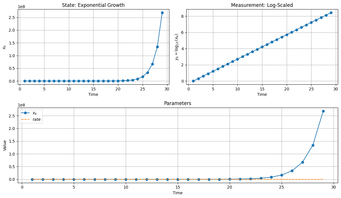
Consider the following example, where we bind the \((f,h)\) representation of a standard exponential growth model.

from pykal import DynamicalSystem


def f(xk: float, rate: float = 1):
    """
    Discrete-time exponential growth model.

    x_{k+1} = rate * x_k
    """
    xk_next = rate * xk
    return xk_next


def h(xk: float):
    """
    Measurement model (identity and scaled by log 10).
    """
    return np.log10(xk)


# Although mathematically, f and h have the same parameters, in our software implementation we need only include those paramters for f and h that they use. This is for convenience. See "Parameter Binding" for more.


exp_growth = DynamicalSystem(f=f, h=h)
exp_growth.__dict__

{'_f': <function __main__.f(xk: float, rate: float = 1)>,
 '_h': <function __main__.h(xk: float)>}

Note

Although mathematically \(f\) and \(h\) have the same parameters, in our Python definitions of f and h we need only include those paramters which are actually used by the functions. This is for convenience and readability; see “Parameter Binding” for more.

Now that we have bound the \((f,h)\) representation, we need a way to call it. Recall from the preceding sections that we have

\[ (f, h)(x_k,\mu_k) = (x_{k+1},y_k) \]

The DynamicalSystem object we’ve created has only a single method, called step(). The step() method has a keyword argument params= which expects an object of type Dict. When step(params=Dict) is called, the DynamicalSystem object passes the parameters to the bound \((f,h)\) and computes \((f,h)(...) = (x_{k+1},y_k)\).

Consider the following simulation of exponential growth.

import numpy as np

dt = 1.0
T = np.arange(0.0, 30.0, dt)  # time domain

X = []
Y = []
M = []

xk = 1  # initial condition
rate = 2
for tk in T[:-1]:
    xk_next, yk = exp_growth.step(params={"xk": xk, "rate": rate})

    X.append(xk)
    Y.append(yk)
    M.append([xk, rate])

    xk = xk_next

Show code cell source

Hide code cell source

import matplotlib.pyplot as plt

# Convert to arrays
X = np.asarray(X)
Y = np.asarray(Y)
M = np.asarray(M)

# Time alignment: X[k], Y[k], M[k] correspond to T[k+1]
T_plot = T[1:]

# Create ONE figure with THREE plots
fig = plt.figure(figsize=(12, 7))

# ---- Top-left: State ----
ax1 = fig.add_subplot(2, 2, 1)
ax1.plot(T_plot, X, marker="o")
ax1.set_title("State: Exponential Growth")
ax1.set_xlabel("Time")
ax1.set_ylabel(r"$x_k$")
ax1.grid(True)

# ---- Top-right: Measurement ----
ax2 = fig.add_subplot(2, 2, 2)
ax2.plot(T_plot, Y, marker="o")
ax2.set_title("Measurement: Log-Scaled")
ax2.set_xlabel("Time")
ax2.set_ylabel(r"$y_k = \log_{10}(x_k)$")
ax2.grid(True)

# ---- Bottom: x_k and rate ----
ax3 = fig.add_subplot(2, 1, 2)
ax3.plot(T_plot, M[:, 0], label=r"$x_k$", marker="o")
ax3.plot(T_plot, M[:, 1], label=r"$\text{rate}$", linestyle="--")
ax3.set_title("Parameters")
ax3.set_xlabel("Time")
ax3.set_ylabel("Value")
ax3.legend()
ax3.grid(True)

plt.tight_layout()
plt.show()

References and Examples

The power of the \((f,h)\) abstraction lies in its flexibility and composability. In the following sections, we’ll explore:

• Stateless systems vs Stateful systems

• Single step vs simulation loops

• Parameter Binding: (enables flexibility when defining f and h)

• Composing Systems

Stateless vs Stateful

The DynamicalSystem constructor accepts two parameters: f and h. However, the ‘f’ function is optional, and excluding it is occasionally useful.

Stateless System (h only)

A stateless system has no internal state evolution; that is, if we consider the \((f,h)\) representation, then \(f\) is the null function (\(f: \varnothing \rightarrow \varnothing\)). You would be right to question why we should even bother encapsulating such a system in a DynamicalSystem object; indeed, we could simply call the function ‘h’ directly.

However, ‘DynamicalSystem’ objects can be useful for initial control system modeling, and, as we will see in ROS [link], if we want to create a stateless transformation node, then we need to first define a stateless DynamicalSystem object.

# Example: Nonlinear sensor that squares its input
def sensor_h(raw_signal: float) -> float:
    """Quadratic sensor response"""
    return raw_signal**2


sensor = DynamicalSystem(h=sensor_h)


print(f"sensor.f = {sensor.f}")

# Step just calls h
output = sensor.step(params={"raw_signal": 3.0})
print(f"\nSensor output: {output}")

sensor.f = None

Sensor output: 9.0

Stateful System

This is what comes to mind when we think of dynamical systems. A stateful system maintains internal “memory” (i.e. state) and evolves over time. This is where the \((f,h)\) representation shines. The stateful system pattern is the most common for

• Dynamical systems with physics

• Controllers with integral/derivative terms

• Observers/estimators

• Any system with memory

# Example: Simple integrator (accumulator)
def integrator_f(integral_state: float, input_signal: float, dt: float) -> float:
    """Integrate input signal over time"""
    return integral_state + input_signal * dt


def integrator_h(integral_state: float) -> float:
    """Output the accumulated integral"""
    return integral_state


integrator = DynamicalSystem(f=integrator_f, h=integrator_h)


print(f"\nintegrator.f = {integrator.f}")
print(f"\nintegrator.h = {integrator.h}")

integrator.f = <function integrator_f at 0x738e5c013100>

integrator.h = <function integrator_h at 0x738e5c013420>

Tip

States and outputs are not restricted to numbers and vectors. They can be vectors, matrices, tuples, functions, classes, neural networks, strings, or any other Python objects. Just make sure you add function annotations so it is clear what type of objects f and h expect.

Single Step vs Simulation Loops

The step() method calls the \((f,h)\) function with the appropriate parameters. You can think of it as executing one “step” of an iteration.

Single Step

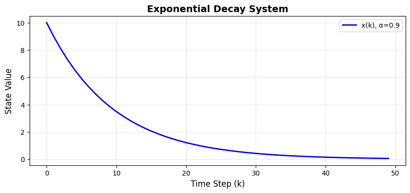
# Simple exponential decay: x_{k+1} = alpha * x_k
def decay_f(xk: float, alpha: float) -> float:
    return alpha * xk


def decay_h(xk):
    return xk


decay_system = DynamicalSystem(f=decay_f, h=decay_h)

# Step
xk = 10
xk_next, yk = decay_system.step(params={"xk": xk, "alpha": 0.9})
print(f"Initial state: {xk}")
print(f"Initial observation: {yk}")
print(f"State after 1 step: {xk_next}")

Initial state: 10
Initial observation: 10
State after 1 step: 9.0

Simulation loop

# Simulate exponential decay for 50 steps
xk = 10.0
alpha = 0.9
steps = 50

X = []
# Y = [] we can include these if we wish
# M = []
for k in range(steps):
    xk_next, y = decay_system.step(params={"xk": xk, "alpha": alpha})

    X.append(xk)
    # Y.append(yk)
    # M.append(alpha) # in this case, we just want to keep track of our paramter alpha

    xk = xk_next

Show code cell source

Hide code cell source

X = np.asarray(X)
# Visualize
plt.figure(figsize=(10, 4))
plt.plot(X, "b-", linewidth=2, label=f"x(k), α={alpha}")
plt.xlabel("Time Step (k)", fontsize=12)
plt.ylabel("State Value", fontsize=12)
plt.title("Exponential Decay System", fontsize=14, fontweight="bold")
plt.grid(True, alpha=0.3)
plt.legend()
plt.show()

Warning

Be mindful of the order in which we call things in the simulation: first (f,h) is called, then X and Y are updated, and finally xk is set to xk_next. This ensures we don’t append xk_next beyond the range of the simulation.

Parameter Binding

As you have likely noticed, although mathematically the parameters for \(f\) and \(h\) are the same, programmatically f and h declare different parameters. What is happening is that the .step(params=Dict) method has a common params dictionary, and relevant parameters for either f or h are routed internally. This is very convenient if parameters are duplicated across functions and makes for more readable code.

Positional vs Keyword Arguments

Functions can use any combination of positional and keyword arguments. The .step() method does not discriminate between them.

The _smart_call Function

Under the hood, the .step() method uses a static method called _smart_call() to route parameters from the shared params dictionary to the appropriate function arguments. This function inspects the signature of f or h, extracts only the parameters each function needs from the dictionary, and calls the function with those parameters.

While _smart_call() is used internally by .step(), advanced users can call it directly when implementing complex algorithms. For example, the Kalman Filter implementation uses _smart_call() within its own f function to invoke the plant’s evolution and measurement functions with the correct parameters.

For technical details on how parameter binding works, see the API reference for _smart_call.

# Different signature styles
def style_1(x: float, u: float) -> float:
    """Positional or keyword arguments"""
    return x + u


def style_2(x: float, *, u: float) -> float:
    """Keyword-only argument (u must be named)"""
    return x + u


def style_3(x: float, u: float, dt: float = 0.1) -> float:
    """With default value"""
    return x + u * dt


def identity_h(x):
    return x


sys1 = DynamicalSystem(f=style_1, h=identity_h)
sys2 = DynamicalSystem(f=style_2, h=identity_h)
sys3 = DynamicalSystem(f=style_3, h=identity_h)

params = {"x": 1.0, "u": 2.0, "dt": 0.5}

# All work with .step()!
print(f"Style 1 result: {sys1.step(params=params)[0]}")  # just print the state
print(f"Style 2 result: {sys2.step(params=params)[0]}")
print(f"Style 3 result: {sys3.step(params=params)[0]}")

# If we omit dt, style_3 uses default (hence, a kwarg proved useful here)
params_no_dt = {"x": 1.0, "u": 2.0}
print(f"Style 3 with default dt: {sys3.step(params=params_no_dt)[0]}")

Style 1 result: 3.0
Style 2 result: 3.0
Style 3 result: 2.0
Style 3 with default dt: 1.2

Using only **kwargs

Functions with **kwargs will accept all parameters from the params dictionary (however, they will need to be extracted by name). This can be a convenient way of defining functions if you don’t want to bother with updating function signatures as you change the parameters the function will use.

# Flexible function that accepts any parameters
def flexible_h(**kwargs) -> float:
    """Use any available parameters"""
    # Extract what we need, with defaults
    a = kwargs.get("a", 1.0)
    b = kwargs.get("b", 0.0)
    c = kwargs.get("c", 0.0)
    x = kwargs.get("x", 0.0)
    return a * x + b * x**2 + c


flexible_sys = DynamicalSystem(h=flexible_h)

# Can provide different parameter combinations (since we have defaults in the definition)
result1 = flexible_sys.step(params={"x": 2.0, "a": 3.0})
result2 = flexible_sys.step(params={"x": 2.0, "a": 3.0, "b": 0.5})
result3 = flexible_sys.step(params={"x": 2.0, "a": 3.0, "b": 0.5, "c": 1.0})

print(f"Result with a only: {result1}")
print(f"Result with a, b: {result2}")
print(f"Result with a, b, c: {result3}")

Result with a only: 6.0
Result with a, b: 8.0
Result with a, b, c: 9.0

Parameter Dictionary Sharing

Multiple systems can share a common parameter dictionary. The .step() method extracts only what each function needs.

# System 1 needs only x and a
def sys1_h(x: float, a: float) -> float:
    return a * x


# System 2 needs only y and b
def sys2_h(y: float, b: float) -> float:
    return b * y


system_a = DynamicalSystem(h=sys1_h)
system_b = DynamicalSystem(h=sys2_h)

# Shared parameter dictionary with all parameters
shared_params = {
    "x": 2.0,
    "y": 3.0,
    "a": 1.5,
    "b": 2.0,
    "unused_param": 999,  # Ignored by both systems
}

result_a = system_a.step(params=shared_params)
result_b = system_b.step(params=shared_params)

print(f"System A extracts (x, a): {result_a}")
print(f"System B extracts (y, b): {result_b}")

System A extracts (x, a): 3.0
System B extracts (y, b): 6.0

Warning

Names are everything! Be consistent with your naming. Nine times out of ten, when there are issues with this package, it is because the user was not careful with naming their parameters.

Composition

The real power of the DynamicalSystem emerges when we compose multiple systems. See Example: Car Cruise Control.

Casting Algorithms in an \((f,h)\)-representation

It’s one thing to prove that any algorithm has an \((f,h)\)-representation–it’s another thing to actually create and use such a representation. See Example: Kalman Filter for an example on how to do so with a classic state estimation algorithm.

← Modules