← Control Systems as Dynamical Systems
Example: Car Cruise Control
Suppose we want to build a robot. If we were hobbyists, we might want a weekend project; if we were engineers, we might need an extra arm on the assembly line; if we were academics, we might dream of a quadruped with a cannon-head to threaten the government for grant money.
Of course, we must begin somewhere. In this notebook, we take a classic example of a feedback system – a car with cruise control – and use pykal to take it from a block diagram to a composition of dynamical systems.
System Overview
We consider here a gross simplification: our car will only ever drive on a perfectly flat plane with minimal drag.
We are given an acceleromoter (which will give us a measurement of our current speed), a button on the steering wheel (which will enable us to modify the cruise control speed), and the car’s CPU (i.e. we can implement any algorithm we want).
Dynamical System Graph
Warning
This section assumes you have already gone through the Dynamical System notebook. If you have not, please do so now.
Recall the following block diagram for a simple feedback system:

where \(r\) is the setpoint (or reference point), \(u\) is the control input, \(x\) is the (hidden) state of the plant, \(\hat{x}\) is the state estimate, and \(e\) is the error term.
In the case of our car cruise control system, we can leverage this diagram with a simple relabling:

where the PID is a proportional-integrative-differential control algorithm, KF is a Kalman filter, and the car is, well, the car.
Note
If you were to ask five control theorists to design a block diagram, you would get six different diagrams. Don’t fret the particulars; the diagram is simply a tool to organize our thinking.
We now proceed with casting the block diagram defined above as dynamical system graph:

We construct this graph block-by-block in the sections that follow.
Note
Although the signals between blocks have remained, for the most part, unchanged, the summing junction and inverter have dissapeared. Indeed, they’ve been absorbed into the PID block, as our implementation of the algorithm computes the error term internally.
Block 1: Setpoint Generator

The setpoint generator maintains the cruise control speed reference based on the driver’s button inputs.
# ---- SETPOINT BLOCK ---------------------

#### ARROWS IN ####
bk = int  # button input; bk in {-1, 0, 1} (decrement, neutral, increment)

#### PARAMETERS ############
sk = int
bk = int  # Current setpoint state (cruise control setpoint in mph)

#### ARROWS OUT ####
rk = float

# ---- $(f,h)$-representation --------------

from pykal import DynamicalSystem


def setpoint_f(sk: float, bk: int) -> float:
    """Increment or decrement setpoint based on button input."""
    return sk + bk


def setpoint_h(
    sk: float,
) -> float:
    """Return the current setpoint speed."""
    rk = sk
    return rk


setpoint_block = DynamicalSystem(f=setpoint_f, h=setpoint_h)
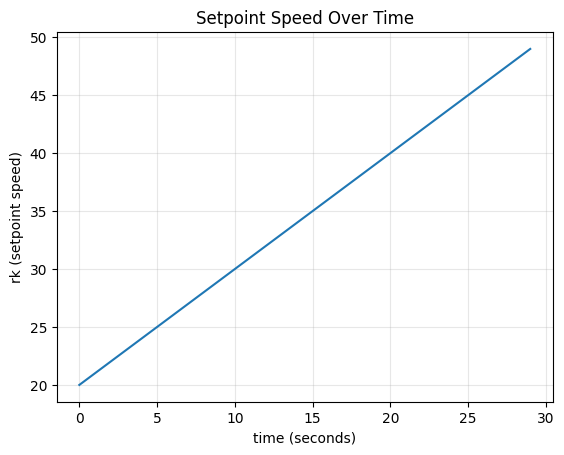
To get a feel for our setpoint dynamical system, we simulate the following scenario: we press up on the button once a second for 30 seconds.
import numpy as np

# ---- SETPOINT GENERATOR BLOCK -------------------

#### ARROWS IN #########################
bk = 1

#### PARAMETERS #########################
sk = 20
bk = bk

#### ARROWS OUT #########################
rk = None
# ---- -------------------

### SIMULATION VARIABLES ############
dt = 1
sim_time = np.arange(0, 30, dt)
rk_hist = []

### SIMULATION ###################################################
for tk in sim_time:
    sk_next, rk = setpoint_block.step(params={"sk": sk, "bk": bk})
    sk = sk_next

    rk_hist.append(rk)
Simulating Different Scenarios
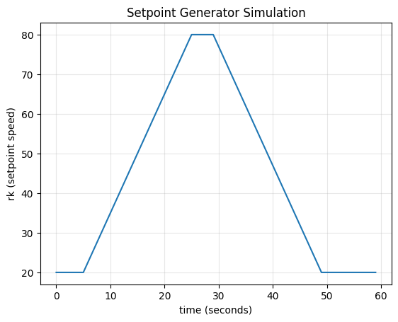
We are limited only by our creativity. Here, we simulate the following scenario:
“Our initial setpoint speed is 20 mph. After five seconds, we feel bold and hold “up” on the cruise control button. Since we are holding the button, the button does not increment the speed setpoint once per second but instead at a rate of three times a second (many buttons have a such feature).
Out cruise control maxes out at 80 mph. Once we reach our maximum setpoint speed, we maintain it for five seconds until we wiener out – at which point, we hold “down” on the cruise control button, which decrements three times a second until our setpoint is back at 20 mph.”
We can model this scenario easily (note that we are still focusing on the setpoint speed, not the actual speed of the car; that will come later).
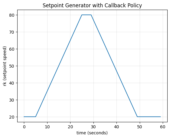
Not too shabby. This seems like a fun scenario to play with, so we will keep it around. But for the sake of convenience, we can compose the button logic above into another DynamicalSystem object.
Composing Dynamical Systems
We will call the scenario defined above, somewhate unimaginatively, as “scenario_1”. After some thinking, we can cast the button logic in the scenario in an \((f,h)\)-representation.
We define a “Scenario 1” block and update our diagram as follows:

Now we have a much cleaner simulation of our scenario above.
Note
We immediately become less formal; going forward, we only will declare and initialize variables which must be defined prior to the simulation, and we will only define them once. This is to reduce code clutter and improve readability.
To make this even more succinct, we can wrap the composition of dynamical systems above into yet another dynamical system, which we will call the “scenario_1_setpoint_generator”.

Note
The blue box represents wrapped dynamical system blocks. Internally, it contains two subsystems that communicate via signals, but externally it presents a simpler interface
We now have a wonderfully minimal interface to play with!
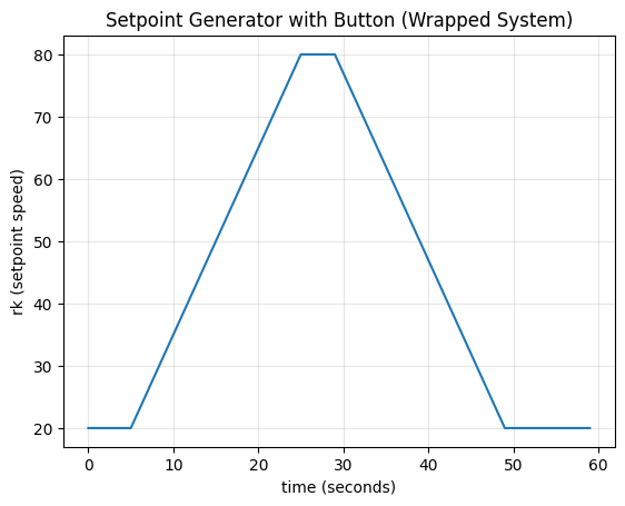
✓ Wrapped system produces the same result with much simpler code!
Block 2: PID

The PID controller compares the setpoint to the estimated state and computes a control command to minimize tracking error. To see the derivation of the evolution and output functions, click on the notebook link in the preceding sentence.
To get a feel for the PID controller, we create a simple mock system and simulate scenario_1.
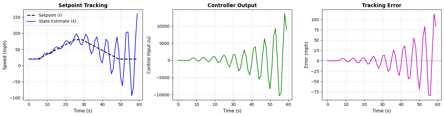
Yikes! Looks like our PID gains are incorrect. Can you fix them? And if you’re able to fix them, see what happens when you change some parameters for scen_1_setpoint_block. Is your fix robust?
Block 3: Car (Plant)

The car dynamics are modeled with position and velocity as the state, and linear drag acting on the velocity.
We can now update our previous PID controller simulation with the actual system we’re controlling!
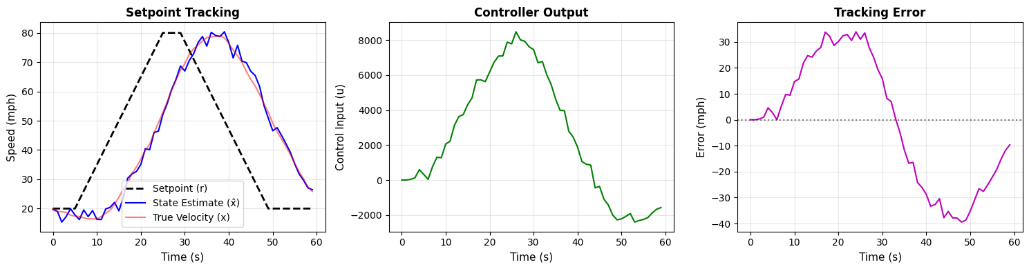
Alas! Can you tune the gains here? And how does changing the mass or drag of the car affect the optimal gains?
Block 4: KF (Observer)

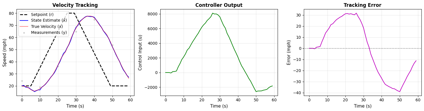
The Kalman filter estimates the car’s velocity by fusing the motion model with noisy measurements.
We can now simulate the full system.
Wrapping the Complete System
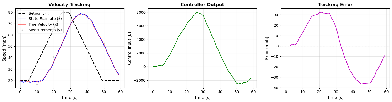
Just as we wrapped the button logic into a DynamicalSystem earlier, we can wrap the entire cruise control system into a single DynamicalSystem object. All system parameters can be configured at initialization, and the simulation loop becomes trivial.

The diagram above shows the complete cruise control system in two views. The top view shows all five subsystems (Button, Setpoint, PID, Plant, and Observer) wrapped inside a blue box, with all internal signals visible. The bottom view shows the same system from the outside—a single DynamicalSystem block with a clean interface that accepts parameters and returns the desired variables.
With the state as we’ve defined it, initialization might seem tricky. Here we introduce a neat trick to make initialization trivial: we can run the previous simulation once and set the appropriate values in \(C_k\)!
import numpy as np

rng = np.random.default_rng()

### SIMULATION VARIABLES ############
dt = 1
sim_time = np.arange(0, 60, dt)

Qk = np.array([[1e-1, 0], [0, 2e-1]])  # add process and measurement noise
Rk = np.array([[3]])

rk_hist = []
uk_hist = []
error_hist = []
xhatk_hist = []
xk_hist = []
yk_hist = []

### SIMULATION ###################################################
for tk in sim_time:
    Ck_next, output_dict = cruise_control_block.step(
        params={
            "Ck": Ck,
            "tk": tk,
            "Qk": Qk,
            "Rk": Rk,
            "scen_1_const_params": scen_1_const_params,
            "pid_const_params": pid_const_params,
            "car_const_params": car_const_params,
            "kf_const_params": kf_const_params,
        }
    )

    rk_hist.append(output_dict["rk"])
    uk_hist.append(output_dict["uk"])
    xhatk_hist.append(output_dict["xhatk"])
    xk_hist.append(output_dict["xk"])  # true velocity
    error_hist.append(output_dict["err"])
    yk_hist.append(output_dict["yk"])
Experimentation
Controller tuning:
Adjust PID gains (KP, KI, KD) to reduce overshoot
What happens if you increase KP too much? (oscillations)
What happens if KD is too small? (slow settling)
Find optimal gains for minimal overshoot and settling time
Setpoint policy:
Change button policy parameters (button_rate, hold_seconds_at_max)
Try different target speeds and ramp rates
Design a smooth sinusoidal setpoint trajectory
Plant variations:
Modify physical parameters (m, b) to simulate different vehicles
Heavy truck: m=5000 kg, b=100 kg/s
Sports car: m=1000 kg, b=30 kg/s
Add measurement noise to make the problem more realistic
Tune Kalman filter covariances (Q, R) for different noise scenarios
Challenge: Can you design PID gains that work well for both a heavy truck and a sports car?