Example: PID Controller

The PID (Proportional-Integral-Derivative) controller is one of the most widely used feedback control algorithms in industrial and robotics applications. This controller adjusts a control input based on three terms to achieve desired system behavior: proportional response to current error, integral action to eliminate steady-state error, and derivative action for damping.

By alternating between error computation, integral accumulation, and derivative estimation, the PID controller produces a control signal that drives the plant output toward the desired setpoint. The controller’s performance depends on careful gain tuning to balance responsiveness, steady-state accuracy, and stability.

For further information, read the Wikipedia article. For the classic paper on PID tuning, see Ziegler and Nichols (1942).

The PID controller dynamical system as implemented in this notebook may be found in the API reference under “Controllers”: PID Controller.

Definition of Algorithm

Notation and Assumptions

We consider a discrete-time control problem where we wish to regulate a plant output $y_k$ to track a reference signal $r_k$. The PID controller computes a control input $u_k$ based on the tracking error $$ e_k = r_k - y_k, $$ where:

$r_k \in \mathbb{R}$ is the reference (setpoint) at time step $k$,
$y_k \in \mathbb{R}$ is the measured plant output,
$e_k \in \mathbb{R}$ is the tracking error.

The discrete-time PID control law is given by $$ u_k = K_P e_k + K_I I_k + K_D (e_k - e_{k-1}), $$ where:

$K_P$ is the proportional gain,
$K_I$ is the integral gain,
$K_D$ is the derivative gain,
$I_k$ is the accumulated integral of error,
$e_{k-1}$ is the previous error.

The integral term evolves according to $$ I_{k+1} = I_k + e_k. $$

How it works

The PID controller combines three control actions to achieve desired system performance:

Proportional Term

The proportional term $K_P e_k$ provides immediate corrective action proportional to the current error. A larger proportional gain increases responsiveness and reduces rise time, but excessive gain can cause overshoot and sustained oscillations. This term provides the primary driving force toward the setpoint.

Integral Term

The integral term $K_I I_k$ accumulates past tracking errors over time. This accumulation ensures that steady-state errors are eventually eliminated, even in the presence of constant disturbances or model uncertainties. The integral action drives the steady-state error to zero by continuing to increase the control effort as long as any error persists. However, excessive integral gain can cause overshoot and slow oscillations, and the accumulation of error during transients can lead to integral windup when control limits are reached.

Derivative Term

The derivative term $K_D (e_k - e_{k-1})$ responds to the rate of change of the tracking error, providing anticipatory control action. This term acts as a predictor of future error trends, adding damping to reduce overshoot and improve stability. The derivative action opposes rapid changes in the plant output, smoothing the system response. However, because it amplifies high-frequency content, the derivative term can be sensitive to measurement noise and may require filtering in practice.

Combined Action

Together, these three terms provide a versatile control strategy: the proportional term drives toward the setpoint, the integral term eliminates steady-state offset, and the derivative term provides damping and reduces overshoot. The relative weighting of these terms (the gains $K_P$, $K_I$, $K_D$) determines the closed-loop performance and must be selected through tuning.

For details on Ziegler-Nichols tuning, see the original paper or this tutorial.

Algorithm as an $(f,h)$-representation

To represent the PID controller as a discrete-time dynamical system, we define the algorithm state to be the tuple $$ c_k := (e_k, I_k, e_{k-1}), $$ where:

$e_k \in \mathbb{R}$ is the current tracking error,
$I_k \in \mathbb{R}$ is the accumulated integral of error,
$e_{k-1} \in \mathbb{R}$ is the previous error (for derivative computation).

The controller is driven by inputs $(r_k, \hat{x}_k)$ where:

$r_k$ is the reference (setpoint),
$\hat{x}_k$ is the measured (or estimated) plant output.

With this setup, the PID controller is the recursion $$ c_{k+1} = f(c_k, r_k, \hat{x}_k; \theta), $$ where $\theta = (K_P, K_I, K_D)$ are the controller gains. The state transition function $f$ computes:

Error computation $$ e_k = r_k - \hat{x}_k. $$

Integral update $$ I_{k+1} = I_k + e_k. $$

State update $$ c_{k+1} = (e_k, I_{k+1}, e_k). $$

The controller output (control input to the plant) is $$ u_k = h(c_k, r_k, \hat{x}_k; \theta) = K_P e_k + K_I I_k + K_D (e_k - e_{k-1}). $$

In pykal, this corresponds to:

State transition: f(...) implements the state evolution, taking the current state and inputs and returning the next state.
Output map: h(...) implements the control law, computing the control input $u_k$ from the current state and gains.

from typing import Tuple
from numpy.typing import NDArray


def f(
    *,
    ck: Tuple[float, float, float],
    rk: float,
    xhat_k: float) -> Tuple[float, float, float]:
    """
    Perform one step of the PID controller state evolution.

    Parameters
    ----------
    ck : Tuple[float, float, float]
        Current controller state ``(e_k, I_k, e_{k-1})``:
            - ``e_k``     : current tracking error
            - ``I_k``     : accumulated integral of error
            - ``e_{k-1}`` : previous error (for derivative)

    rk : float
        Reference (setpoint) at time k.

    xhat_k : float
        Measured or estimated plant output at time k.

    Returns
    -------
    Tuple[float, float, float]
        Updated controller state ``(e_{k+1}, I_{k+1}, e_k)``:
            - ``e_{k+1}`` : new tracking error
            - ``I_{k+1}`` : updated integral
            - ``e_k``     : current error (becomes previous error for next step)

    Notes
    -----
    This function implements the PID controller state transition:

    Error computation:
        ``e_k = rk - xhat_k``

    Integral update:
        ``I_{k+1} = I_k + e_k``

    State update:
        ``ck_new = (e_k, I_{k+1}, e_k)``

    The control output is computed separately by the ``h`` function.
    """
    e_k_prev, I_k, _ = ck
    
    # Compute current error
    e_k = rk - xhat_k
    
    # Update integral
    I_k_new = I_k + e_k
    
    # Return updated state: (current_error, new_integral, prev_error)
    return (e_k, I_k_new, e_k_prev)


def h(
    *,
    ck: Tuple[float, float, float],
    rk: float,
    xhat_k: float,
    KP: float,
    KI: float,
    KD: float) -> float:
    """
    Compute the PID control output.

    Parameters
    ----------
    ck : Tuple[float, float, float]
        Current controller state ``(e_k, I_k, e_{k-1})``.

    rk : float
        Reference (setpoint) at time k.

    xhat_k : float
        Measured or estimated plant output at time k.

    KP : float
        Proportional gain.

    KI : float
        Integral gain.

    KD : float
        Derivative gain.

    Returns
    -------
    float
        Control input ``u_k`` to be applied to the plant.

    Notes
    -----
    This function implements the standard PID control law:

    Error:
        ``e_k = rk - xhat_k``

    Control output:
        ``u_k = KP * e_k + KI * I_k + KD * (e_k - e_{k-1})``

    The control output combines:
    - Proportional term: responds to current error
    - Integral term: eliminates steady-state error
    - Derivative term: provides damping based on error rate
    """
    e_k_prev, I_k, e_k_old = ck
    
    # Compute current error
    e_k = rk - xhat_k
    
    # PID control law
    u_k = KP * e_k + KI * I_k + KD * (e_k - e_k_old)
    
    return u_k

Example: First-Order System Tracking

We demonstrate the PID controller on a simple first-order system (representing a DC motor, thermal system, or RC circuit). The controller tracks step changes in the setpoint, demonstrating its ability to achieve zero steady-state error and reject disturbances.

We consider the continuous-time first-order system $$ \dot{x}(t) = -a x(t) + b u(t), $$ where $x(t)$ is the state, $u(t)$ is the control input, $a > 0$ is the decay rate (inverse time constant), and $b > 0$ is the control gain.

Using Euler discretization with time step $\Delta t$, we obtain $$ x_{k+1} = x_k + \Delta t(-a x_k + b u_k). $$

The output is the state itself: $y_k = x_k$.

Note that even though this is a simple first-order system, the PID controller must account for both immediate error (P term), accumulated error (I term), and error rate (D term) to achieve good tracking performance. This demonstrates the controller’s versatility across different system dynamics.

The diagram above shows the closed-loop control structure: the reference $r_k$ is compared with the measured output (feedback) to compute the error $e_k$. The PID Controller block maintains internal state $c_k = (e_k, I_k, e_{k-1})$ and computes the control input $u_k$. The Plant block represents the system being controlled (with state $x_k$), which produces the output $y_k$ that is fed back for error computation.

from pykal import DynamicalSystem
import numpy as np
import matplotlib.pyplot as plt

def plant_f(x, u, a, b, dt):
    """
    First-order system state evolution.
    
    Parameters:
        x: Current state (scalar)
        u: Control input (scalar)
        a: Decay rate parameter
        b: Control gain parameter
        dt: Time step
    
    Returns:
        Next state (scalar)
    """
    return x + dt * (-a * x + b * u)


def plant_h(x):
    """
    Plant output function.
    
    Parameters:
        x: Current state (scalar)
    
    Returns:
        Output (state itself)
    """
    return x


plant = DynamicalSystem(f=plant_f, h=plant_h)
controller = DynamicalSystem(f=f, h=h)

# Simulation parameters
dt = 0.01  # Time step (10 ms)
T = 10.0   # Total time (10 seconds)
time = np.arange(0, T, dt)
N = len(time)

# Plant parameters
a = 2.0  # Decay rate
b = 3.0  # Control gain

# Calculate Ziegler-Nichols PID gains
K_system = b / a           # System gain: 1.5
tau_system = 1 / a         # Time constant: 0.5 s

KP = 1.2 / K_system        # 0.8
KI = 2 * KP / tau_system   # 3.2
KD = KP * tau_system / 2   # 0.2

print(f"System parameters: K = {K_system:.2f}, τ = {tau_system:.2f} s")
print(f"PID gains (Ziegler-Nichols): KP = {KP:.3f}, KI = {KI:.3f}, KD = {KD:.3f}")

# Initial conditions
x0 = 0.0                    # Plant starts at zero
ck0 = (0.0, 0.0, 0.0)       # Controller: (error, integral, prev_error)

# Storage
x_history = []
u_history = []
r_history = []
ck_history = []

# Initial state
xk = x0
ck = ck0

System parameters: K = 1.50, τ = 0.50 s
PID gains (Ziegler-Nichols): KP = 0.800, KI = 3.200, KD = 0.200

# Closed-loop simulation
for k, tk in enumerate(time):
    # Update setpoint (step changes)
    if tk < 3.0:
        rk = 1.0
    elif tk < 6.0:
        rk = 2.0
    else:
        rk = 0.5
    
    # Measure plant output (perfect measurement)
    yk = plant.h(x=xk)
    
    # Controller computes control input and updates state
    ck, uk = controller.step(
        params={
            'ck': ck,
            'rk': rk,
            'xhat_k': yk,
            'KP': KP,
            'KI': KI,
            'KD': KD
        }
    )
    
    # Apply control to plant
    xk = plant.f(x=xk, u=uk, a=a, b=b, dt=dt)
    
    # Store history
    x_history.append(yk)
    u_history.append(uk)
    r_history.append(rk)
    ck_history.append(ck)

# Convert to arrays
x_history = np.array(x_history)
u_history = np.array(u_history)
r_history = np.array(r_history)
e_history = r_history - x_history

print("Simulation complete!")

Simulation complete!

fig, axes = plt.subplots(3, 1, figsize=(12, 9))

# Plot 1: Output tracking
axes[0].plot(time, r_history, 'r--', linewidth=2, label='Setpoint $r(t)$')
axes[0].plot(time, x_history, 'b-', linewidth=1.5, label='Output $y(t)$')
axes[0].set_ylabel('Output', fontsize=11)
axes[0].set_title('PID Control: First-Order System Tracking', fontsize=13, fontweight='bold')
axes[0].legend(fontsize=10)
axes[0].grid(True, alpha=0.3)

# Plot 2: Control input
axes[1].plot(time, u_history, 'g-', linewidth=1.5, label='Control $u(t)$')
axes[1].set_ylabel('Control Input $u(t)$', fontsize=11)
axes[1].legend(fontsize=10)
axes[1].grid(True, alpha=0.3)

# Plot 3: Tracking error
axes[2].plot(time, e_history, 'm-', linewidth=1.5, label='Error $e(t)$')
axes[2].axhline(y=0, color='k', linestyle=':', alpha=0.3)
axes[2].set_ylabel('Tracking Error $e(t)$', fontsize=11)
axes[2].set_xlabel('Time (seconds)', fontsize=11)
axes[2].legend(fontsize=10)
axes[2].grid(True, alpha=0.3)

plt.tight_layout()
plt.show()

# Performance metrics
print("\nPerformance Metrics:")
print(f"  Final tracking error: {e_history[-1]:.6f}")
print(f"  Max control effort: {np.max(np.abs(u_history)):.3f}")
print(f"  RMS tracking error: {np.sqrt(np.mean(e_history**2)):.6f}")

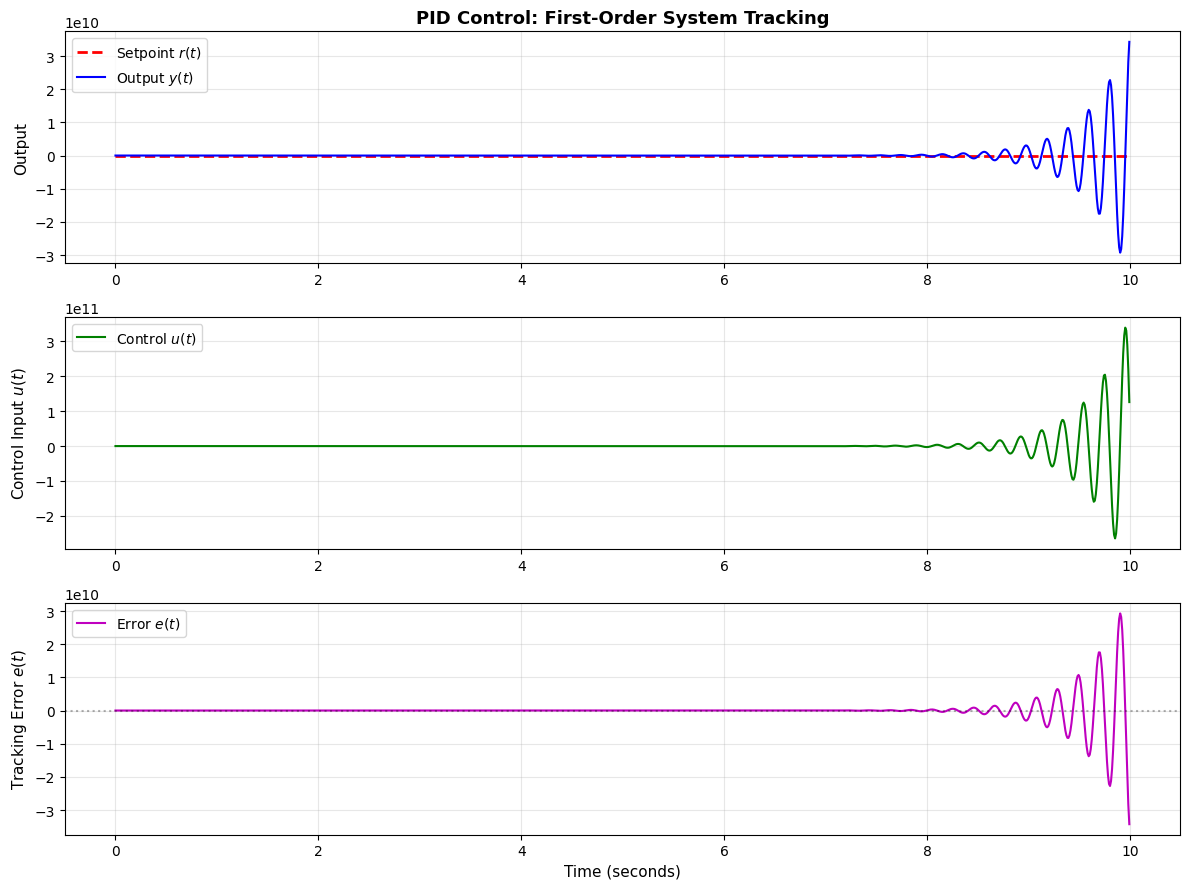
../../_images/40d66b458aecf4e26a91d4c532b2520ea9c0494d684622a62d7c6d8c103d6f0a.png

Performance Metrics:
  Final tracking error: -34268741053.280994
  Max control effort: 339319843282.406
  RMS tracking error: 3695557204.110165

Notes on Usage

The PID controller is appropriate when most of the following conditions hold:

Single-input single-output (SISO) system: PID works best for controlling one output with one input
Stable or marginally stable plant: The open-loop system should not be highly unstable
Smooth dynamics: The plant responds reasonably to control inputs without excessive delays
Measurement availability: The output (or an estimate) can be measured frequently

If your system is multivariable (MIMO), consider using LQR, MPC, or decoupled PID loops. If your system has significant nonlinearities, consider gain scheduling, adaptive control, or nonlinear control methods. For optimal control with constraints, use MPC instead.

Common Applications

The PID controller is widely used in:

Industrial process control: Temperature, pressure, flow, level control
Robotics: Motor speed/position control, altitude control for drones
Automotive: Cruise control, engine control
HVAC systems: Temperature and humidity regulation
Manufacturing: CNC machines, assembly line automation

Tuning Guidance

The performance of the PID controller depends critically on the gain selection:

Proportional gain $K_P$: Larger values → faster response but more overshoot and oscillations
Integral gain $K_I$: Larger values → faster steady-state error elimination but more overshoot and potential instability
Derivative gain $K_D$: Larger values → more damping and reduced overshoot but amplifies measurement noise

Tuning methods:

Ziegler-Nichols: Use step response or ultimate gain method (see original paper)
Cohen-Coon: Better for systems with dead time
Manual tuning: Start with $K_I = K_D = 0$, increase $K_P$ until oscillations, then add $K_D$ for damping and $K_I$ to eliminate offset
Model-based: If plant model is known, use pole placement or optimization

For a practical guide to PID tuning, see this tutorial.

Implementation Details

State representation: The controller state is a tuple (e_k, I_k, e_{k-1}) where:

e_k: current tracking error
I_k: accumulated integral
e_{k-1}: previous error for derivative

Controller inputs: The controller requires:

rk: reference signal (setpoint)
xhat_k: measured or estimated plant output

Derivative on measurement: This implementation computes the derivative on the error. An alternative is to compute the derivative on the measurement only (to avoid derivative kick when setpoint changes). This can be implemented by modifying the h function to use -(xhat_k - xhat_{k-1}) instead of (e_k - e_{k-1}).

Anti-windup: This basic implementation does not include anti-windup protection. For systems with control input saturation, consider adding integral clamping or back-calculation to prevent windup.

Filtering: For noisy measurements, consider low-pass filtering the derivative term or using a filtered derivative approximation.

← Algorithms as Dynamical Systems