DataChange

The data_change module provides tools to model realistic sensor data. In particular, it allows you to:

Corrupt ideal signals to simulate realistic hardware behavior via the data_change.corrupt subclass
Clean corrupted signals for downstream use in estimators and controllers via the data_change.clean subclass

This notebook demonstrates all corruption and preparation methods available in pykal.data_change, using visual examples to illustrate how each transformation affects the underlying signal.

References and Examples

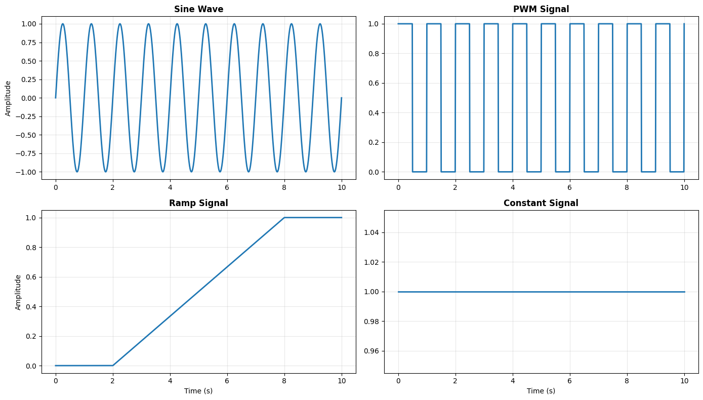
We first generate a representative set of reference signals using the DynamicalSystem class. In the remaining sections, we demonstrate corrupting these signals via

Gaussian noise (thermal noise / ADC noise)
Bias offsets (uncalibrated zero errors)
Drift (time-varying bias from warm-up / temperature)
Quantization (finite ADC resolution)
Spikes / outliers (EMI glitches, electrical transients)
Clipping / saturation (sensor range limits)
Packet loss / dropouts (missing samples, intermittent links)
Contact bounce (encoders, switches, digital edges)
Latency / delay (communication + processing lag)

and then, when cleaning operations are available, demonstrating how to clean the corrupted signals, using such methods as

moving average / low-pass filtering (noise suppression)
median filtering (outlier rejection without blurring edges)
exponential smoothing (real-time filtering)
debouncing (stable digital transitions)
outlier handling (replace or interpolate)
interpolation (filling missing samples)
staleness policies for asynchronous sensors (hold/zero/drop/none)
calibration (bias + scale correction)

Generate Reference Signals

import numpy as np
import matplotlib.pyplot as plt
from pykal import DynamicalSystem

# -----------------------------
# Reference signals (stateless)
# -----------------------------


def sine_wave(tk: float, f_hz: float, amplitude: float, phase: float) -> float:
    """y(t) = A sin(2π f t + φ)"""
    return amplitude * np.sin(2.0 * np.pi * f_hz * tk + phase)


def ramp(tk: float, t0: float, t1: float, y0: float, y1: float) -> float:
    """Linear ramp from (t0, y0) to (t1, y1), clamped outside interval."""
    if tk <= t0:
        return y0
    if tk >= t1:
        return y1
    s = (tk - t0) / (t1 - t0)
    return (1.0 - s) * y0 + s * y1


def constant(c: float) -> float:
    """y(t) = c"""
    return c


def pwm(tk: float, f_hz: float, duty: float, low: float, high: float) -> float:
    """
    Pulse-width modulation (PWM).
    """
    T = 1.0 / f_hz
    phase = tk % T
    return high if phase < duty * T else low


# Wrapping signals in DynamicalSystem objects
ref_sine_wave = DynamicalSystem(h=sine_wave)
ref_constant = DynamicalSystem(h=constant)
ref_ramp = DynamicalSystem(h=ramp)
ref_pwm = DynamicalSystem(h=pwm)

# Simulating signals over time

T = np.linspace(0, 10, 1000)

Y_sin = []
Y_const = []
Y_ramp = []
Y_pwm = []

for tk in T:
    Y_sin.append(
        ref_sine_wave.step(
            params={"tk": tk, "f_hz": 1.0, "amplitude": 1.0, "phase": 0.0}
        )
    )
    Y_const.append(ref_constant.step(params={"c": 1}))
    Y_ramp.append(
        ref_ramp.step(params={"tk": tk, "t0": 2.0, "t1": 8.0, "y0": 0.0, "y1": 1.0})
    )
    Y_pwm.append(
        ref_pwm.step(
            params={"tk": tk, "f_hz": 1.0, "duty": 0.5, "low": 0.0, "high": 1.0}
        )
    )

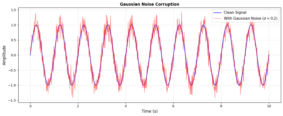
../../../_images/cd94519ae066eeafd2ce66922b3730d8880fc1e14a96d2e62a0aec3105e544b7.png

Gaussian Noise

Thanks to the Central Limit Theorem, sensor noise can often be modeled as the true sensor value plus zero-mean Gaussian noise. That is, the noisy output of the sensor, which we denote $\tilde{y}_k$, is

\[ \tilde{y}_k = y_k + r_k \]

where $r_k \sim \mathcal{N}\bigl(0,\, \sigma \bigr)$.

API reference: pykal.data_change.corrupt.with_gaussian_noise().

from pykal.data_change import corrupt, clean

Y_clean_sin = []
Y_noisy_sin = []

for tk in T:
    yk = ref_sine_wave.step(
        params={"tk": tk, "f_hz": 1.0, "amplitude": 1.0, "phase": 0.0}
    )
    yk_corrupted = corrupt.with_gaussian_noise(yk, mean=0.0, std=0.2)

    Y_clean_sin.append(yk)
    Y_noisy_sin.append(yk_corrupted)

../../../_images/b204886ea19622ae9b38f19d93a74149a7314383037c4dd2539e6dbcaa9bde45.png

Original std:  0.7068
Corrupted std: 0.7247
Noise added:   0.1977

Multivariate Gaussian Noise (with covariance matrix):

For vector-valued sensors (e.g., 3-axis IMU), noise is often correlated across channels. The noisy measurement is

\[ \tilde{\mathbf{y}}_k = \mathbf{y}_k + \mathbf{r}_k \]

where $\mathbf{r}_k \sim \mathcal{N}(\mathbf{0}, \mathbf{Q})$ and $\mathbf{Q}$ is the covariance matrix capturing both individual channel noise levels and cross-channel correlations.

API reference: pykal.data_change.corrupt.with_gaussian_noise() (with Q parameter).

# 3D IMU example: accelerometer with different noise per axis
# Covariance: x low noise, y medium, z high (with small correlations)
Q = np.array([[0.01, 0.002, 0.0], [0.002, 0.05, 0.01], [0.0, 0.01, 0.1]])

# Generate 100 samples from three reference signals
T_imu = np.linspace(0, 10, 100)
IMU_clean = []
IMU_noisy = []

for i, tk in enumerate(T_imu):
    # Generate clean 3D signal (sine, ramp, constant)
    x_clean = ref_sine_wave.step(
        params={"tk": tk, "f_hz": 1.0, "amplitude": 1.0, "phase": 0.0}
    )
    y_clean = ref_ramp.step(
        params={"tk": tk, "t0": 2.0, "t1": 8.0, "y0": 0.0, "y1": 1.0}
    )
    z_clean = ref_constant.step(params={"c": 1})

    clean_vec = np.array([x_clean, y_clean, z_clean])
    # Apply multivariate Gaussian noise in the loop
    noisy_vec = corrupt.with_gaussian_noise(clean_vec, Q=Q, seed=i)

    IMU_clean.append(clean_vec)
    IMU_noisy.append(noisy_vec)

---------------------------------------------------------------------------
TypeError                                 Traceback (most recent call last)
Cell In[5], line 22
     20 clean_vec = np.array([x_clean, y_clean, z_clean])
     21 # Apply multivariate Gaussian noise in the loop
---> 22 noisy_vec = corrupt.with_gaussian_noise(clean_vec, Q=Q, seed=i)
     24 IMU_clean.append(clean_vec)
     25 IMU_noisy.append(noisy_vec)

TypeError: corrupt.with_gaussian_noise() got an unexpected keyword argument 'Q'

Moving Average Filter

The moving average filter smooths noisy signals by replacing each sample with the average of its neighbors:

\[ \hat{y}_k = \frac{1}{w} \sum_{i=0}^{w-1} \tilde{y}_{k-i} \]

where $w$ is the window size. This reduces high-frequency noise but introduces phase lag proportional to $w/2$.

Best for: reducing Gaussian noise Tradeoff: introduces lag, reduces bandwidth

API reference: pykal.data_change.clean.with_moving_average().

T_ma = np.linspace(0, 10, 1000)
Y_original = []
Y_noisy = []
Y_smoothed = []

for tk in T_ma:
    yk = ref_sine_wave.step(
        params={"tk": tk, "f_hz": 1.0, "amplitude": 1.0, "phase": 0.0}
    )
    yk_noisy = corrupt.with_gaussian_noise(yk, std=0.3)

    Y_original.append(yk)
    Y_noisy.append(yk_noisy)

# Apply moving average after generation
Y_noisy_arr = np.array(Y_noisy)
Y_smoothed = clean.with_moving_average(Y_noisy_arr, window=10)

Exponential Smoothing

Exponential smoothing is a recursive filter ideal for real-time applications:

\[ \hat{y}_k = \alpha \tilde{y}_k + (1 - \alpha) \hat{y}_{k-1} \]

where $\alpha \in [0,1]$ controls the smoothing strength. Larger $\alpha$ responds faster but smooths less; smaller $\alpha$ provides more smoothing but reacts slower to changes.

Best for: real-time filtering Parameter: $\alpha \in [0,1]$

API reference: pykal.data_change.clean.with_exponential_smoothing().

T_exp = np.linspace(0, 10, 1000)
Y_clean_exp = []
Y_noisy_exp = []
Y_smoothed_03 = []
Y_smoothed_05 = []
Y_smoothed_08 = []

# Initialize exponential smoothing state for each alpha
y_prev_03 = 0.0
y_prev_05 = 0.0
y_prev_08 = 0.0

for tk in T_exp:
    yk = ref_sine_wave.step(
        params={"tk": tk, "f_hz": 1.0, "amplitude": 1.0, "phase": 0.0}
    )
    yk_noisy = corrupt.with_gaussian_noise(yk, std=0.25)

    # Apply exponential smoothing in the loop (recursive)
    y_smooth_03 = 0.3 * yk_noisy + (1 - 0.3) * y_prev_03
    y_smooth_05 = 0.5 * yk_noisy + (1 - 0.5) * y_prev_05
    y_smooth_08 = 0.8 * yk_noisy + (1 - 0.8) * y_prev_08

    # Update previous values
    y_prev_03 = y_smooth_03
    y_prev_05 = y_smooth_05
    y_prev_08 = y_smooth_08

    Y_clean_exp.append(yk)
    Y_noisy_exp.append(yk_noisy)
    Y_smoothed_03.append(y_smooth_03)
    Y_smoothed_05.append(y_smooth_05)
    Y_smoothed_08.append(y_smooth_08)

# Convert to arrays
smoothed_alpha_03 = np.array(Y_smoothed_03)
smoothed_alpha_05 = np.array(Y_smoothed_05)
smoothed_alpha_08 = np.array(Y_smoothed_08)

Low-Pass Filter (First-Order)

A first-order low-pass filter attenuates high-frequency components while passing low frequencies:

\[ \hat{y}_k = \alpha \tilde{y}_k + (1 - \alpha) \hat{y}_{k-1} \]

Equivalent to exponential smoothing, but interpreted in the frequency domain with cutoff frequency $f_c = \alpha f_s / (2\pi)$ where $f_s$ is the sampling rate.

Best for: attenuating high-frequency noise Parameter: $\alpha \in [0,1]$

API reference: pykal.data_change.clean.with_low_pass_filter().

T_lp = np.linspace(0, 10, 1000)
Y_clean_lp = []
Y_noisy_lp = []
Y_filtered = []

# Initialize low-pass filter state
y_prev = 0.0
alpha = 0.1

for tk in T_lp:
    yk = ref_sine_wave.step(
        params={"tk": tk, "f_hz": 1.0, "amplitude": 1.0, "phase": 0.0}
    )
    yk_noisy = corrupt.with_gaussian_noise(yk, std=0.3)

    # Apply low-pass filter in the loop (recursive)
    y_filtered = alpha * yk_noisy + (1 - alpha) * y_prev
    y_prev = y_filtered

    Y_clean_lp.append(yk)
    Y_noisy_lp.append(yk_noisy)
    Y_filtered.append(y_filtered)

# Convert to array
filtered_lp = np.array(Y_filtered)

Contact Bounce

Mechanical switches and encoders exhibit contact bounce—rapid oscillations near transitions before settling to a stable value:

\[\begin{split} \tilde{y}_k = \begin{cases} y_k + A \cdot \text{noise}_k & \text{if } |k - k_{\text{transition}}| < d \\ y_k & \text{otherwise} \end{cases} \end{split}\]

where $A$ is the bounce amplitude and $d$ is the bounce duration in samples. This non-ideal behavior occurs due to mechanical spring forces causing contacts to vibrate.

Hardware source: mechanical switches and encoders that chatter near transitions Common in: digital inputs, rotary encoders, limit switches

API reference: pykal.data_change.corrupt.with_bounce().

T_bounce = np.linspace(0, 4, 400)
Y_step = []
Y_bounced = []

for tk in T_bounce:
    # Generate step signal: 0 before t=2, 1 after
    yk = 0.0 if tk < 2.0 else 1.0

    Y_step.append(yk)

# Apply bounce corruption after generation
step_signal = np.array(Y_step)
bounced_step = corrupt.with_bounce(step_signal, duration=5, amplitude=0.3, seed=42)

Debounce

Debouncing removes contact bounce by requiring signal stability for a minimum duration before accepting a transition:

\[\begin{split} \hat{y}_k = \begin{cases} \tilde{y}_k & \text{if } |\tilde{y}_j - \tilde{y}_{j-1}| < \epsilon \text{ for all } j \in [k-d, k] \\ \hat{y}_{k-1} & \text{otherwise} \end{cases} \end{split}\]

where $\epsilon$ is the stability threshold and $d$ is the minimum stable duration. This implements a form of temporal hysteresis.

Best for: removing contact bounce from digital signals Idea: require stability for a minimum duration before accepting transitions

API reference: pykal.data_change.clean.with_debounce().

T_debounce = np.linspace(0, 4, 400)
Y_step_debounce = []

for tk in T_debounce:
    yk = 0.0 if tk < 2.0 else 1.0
    Y_step_debounce.append(yk)

# Apply bounce and debounce
step_signal = np.array(Y_step_debounce)
bounced_step_2 = corrupt.with_bounce(step_signal, duration=8, amplitude=0.4, seed=46)
debounced = clean.with_debounce(bounced_step_2, threshold=0.2, min_duration=3)

Dropouts (Packet Loss)

Wireless communication and intermittent sensor connections cause random samples to be missing:

\[\begin{split} \tilde{y}_k = \begin{cases} y_k & \text{with probability } (1 - p) \\ \text{NaN} & \text{with probability } p \end{cases} \end{split}\]

where $p$ is the dropout rate. Missing samples are marked as NaN and must be handled by downstream processing.

Hardware source: wireless links, intermittent buses, sensor hiccups Common in: WiFi sensors, BLE devices, multi-robot comms

API reference: pykal.data_change.corrupt.with_dropouts().

T_dropout = np.linspace(0, 10, 1000)
Y_sine_dropout = []
Y_dropped = []

np.random.seed(42)
dropout_rate = 0.2

for tk in T_dropout:
    yk = ref_sine_wave.step(
        params={"tk": tk, "f_hz": 1.0, "amplitude": 1.0, "phase": 0.0}
    )

    # Apply dropout in the loop (probabilistic per-sample)
    if np.random.rand() < dropout_rate:
        yk_dropped = np.nan
    else:
        yk_dropped = yk

    Y_sine_dropout.append(yk)
    Y_dropped.append(yk_dropped)

# Convert to arrays
sine_wave = np.array(Y_sine_dropout)
dropped_sine = np.array(Y_dropped)

Interpolation (Fill Missing Data)

Interpolation fills missing samples (NaN values) using neighboring valid data:

Linear interpolation: $$ \hat{y}_k = y_i + \frac{k - i}{j - i}(y_j - y_i) $$ where $i < k < j$ and $y_i, y_j$ are the nearest valid samples.

Nearest-neighbor interpolation: $$ \hat{y}_k = y_{\arg\min_i |k - i|} $$

Best for: dropouts (NaN values) Methods: linear (smooth), nearest-neighbor (preserves steps)

API reference: pykal.data_change.clean.with_interpolation().

T_interp = np.linspace(0, 10, 1000)
Y_sine_interp = []

for tk in T_interp:
    yk = ref_sine_wave.step(
        params={"tk": tk, "f_hz": 1.0, "amplitude": 1.0, "phase": 0.0}
    )
    Y_sine_interp.append(yk)

# Apply dropouts and interpolation
sine_wave = np.array(Y_sine_interp)
dropped_sine_2 = corrupt.with_dropouts(sine_wave, dropout_rate=0.15, seed=48)
filled_linear = clean.with_interpolation(dropped_sine_2, method="linear")
filled_nearest = clean.with_interpolation(dropped_sine_2, method="nearest")

Asynchronous / Multi-Rate Data

Hardware source: sensors sampling at different rates, non-uniform timing Common in: sensor fusion (IMU @ 100Hz, GPS @ 10Hz, camera @ 30Hz)

# Simulate three sensors with different sampling rates
t_fast = np.arange(0, 2, 0.01)  # 100 Hz
t_medium = np.arange(0, 2, 0.033)  # ~30 Hz
t_slow = np.arange(0, 2, 0.1)  # 10 Hz

# Generate fast sensor data
signal_fast = []
for tk in t_fast:
    yk = np.sin(2 * np.pi * 1.5 * tk)
    signal_fast.append(yk)
signal_fast = np.array(signal_fast)
signal_fast_noisy = corrupt.with_gaussian_noise(signal_fast, std=0.05, seed=60)

# Generate medium sensor data
signal_medium = []
for tk in t_medium:
    yk = np.sin(2 * np.pi * 1.5 * tk)
    signal_medium.append(yk)
signal_medium = np.array(signal_medium)
signal_medium_noisy = corrupt.with_gaussian_noise(signal_medium, std=0.08, seed=61)

# Generate slow sensor data
signal_slow = []
for tk in t_slow:
    yk = np.sin(2 * np.pi * 1.5 * tk)
    signal_slow.append(yk)
signal_slow = np.array(signal_slow)
signal_slow_noisy = corrupt.with_gaussian_noise(signal_slow, std=0.1, seed=62)

Kalman Filter Multi-Rate Sensor Fusion

The optimal solution for fusing asynchronous sensors with different noise characteristics is the Kalman filter. Here we demonstrate:

Fast sensor (100 Hz): High rate but noisy (σ = 0.3)
Slow sensor (10 Hz): Low rate but accurate (σ = 0.05)
Kalman filter: Optimally weights both based on their noise characteristics

from pykal.algorithm_library.estimators.kf import KF

# True state evolution: simple 1D constant velocity
# State: [position, velocity]
dt_sim = 0.01  # Simulation timestep (100 Hz)
t_total = 2.0
t_sim = np.arange(0, t_total, dt_sim)

# True state trajectory
true_pos = np.sin(2 * np.pi * 0.5 * t_sim)  # Sinusoidal position
true_vel = 2 * np.pi * 0.5 * np.cos(2 * np.pi * 0.5 * t_sim)  # Derivative

# Generate sensor measurements
# Fast sensor: measures position every 0.01s (100 Hz) with high noise
fast_noise_std = 0.3
np.random.seed(100)
fast_measurements = true_pos + np.random.normal(0, fast_noise_std, len(t_sim))

# Slow sensor: measures position every 0.1s (10 Hz) with low noise
slow_rate = 10  # Every 10 samples
slow_noise_std = 0.05
slow_measurements = np.full_like(true_pos, np.nan)
slow_measurements[::slow_rate] = true_pos[::slow_rate] + np.random.normal(
    0, slow_noise_std, len(true_pos[::slow_rate])
)

# Kalman filter setup - constant velocity model
# State: x = [position, velocity]^T
# Dynamics: position_{k+1} = position_k + velocity_k * dt
#           velocity_{k+1} = velocity_k


# State transition matrix (constant for linear system)
def get_F(dt):
    return np.array([[1.0, dt], [0.0, 1.0]])


# Measurement matrix (observe position only)
H = np.array([[1.0, 0.0]])

# Process noise covariance
Q = np.diag([0.01, 0.01])

# Measurement noise covariances
R_fast = np.array([[fast_noise_std**2]])
R_slow = np.array([[slow_noise_std**2]])

# Initialize state estimate
x_est = np.array([[0.0], [0.0]])  # Start at origin with zero velocity
P_est = np.diag([1.0, 1.0])  # Initial uncertainty

# Storage
kf_positions = []
kf_velocities = []

# Run Kalman filter
for i in range(len(t_sim)):
    # Predict step (always done)
    F = get_F(dt_sim)
    x_pred = F @ x_est  # State prediction
    P_pred = F @ P_est @ F.T + Q  # Covariance prediction

    # Update step (if measurement available)
    has_slow = not np.isnan(slow_measurements[i])
    has_fast = not np.isnan(fast_measurements[i])

    if has_slow:
        # Use slow (accurate) sensor
        z = np.array([[slow_measurements[i]]])
        R = R_slow
    elif has_fast:
        # Use fast (noisy) sensor
        z = np.array([[fast_measurements[i]]])
        R = R_fast
    else:
        # No measurement - use prediction
        x_est = x_pred
        P_est = P_pred
        kf_positions.append(x_est[0, 0])
        kf_velocities.append(x_est[1, 0])
        continue

    # Kalman gain
    S = H @ P_pred @ H.T + R
    K = P_pred @ H.T @ np.linalg.inv(S)

    # Update estimate
    y_pred = H @ x_pred
    innovation = z - y_pred
    x_est = x_pred + K @ innovation
    P_est = (np.eye(2) - K @ H) @ P_pred

    kf_positions.append(x_est[0, 0])
    kf_velocities.append(x_est[1, 0])

kf_positions = np.array(kf_positions)
kf_velocities = np.array(kf_velocities)

# Compute errors
fast_error_rms = np.sqrt(np.mean((fast_measurements - true_pos) ** 2))
slow_error_rms = np.sqrt(np.nanmean((slow_measurements - true_pos) ** 2))
kf_error_rms = np.sqrt(np.mean((kf_positions - true_pos) ** 2))

print(f"Fast sensor RMS error: {fast_error_rms:.4f}")
print(f"Slow sensor RMS error: {slow_error_rms:.4f}")
print(f"Kalman filter RMS error: {kf_error_rms:.4f}")
print(f"\nImprovement over fast sensor: {(1 - kf_error_rms/fast_error_rms)*100:.1f}%")
print(f"Improvement over slow sensor: {(1 - kf_error_rms/slow_error_rms)*100:.1f}%")

Staleness Policy (Asynchronous Sensors)

Asynchronous sensors arrive at different times, requiring policies for handling missing data:

Policies:

zero: $\hat{y}_k = 0$ if NaN (assumes baseline state)
hold: $\hat{y}_k = \hat{y}_{k-1}$ if NaN (zero-order hold)
drop: remove NaN samples entirely (variable-rate output)
none: keep NaN (downstream must handle)

\[\begin{split} \hat{y}_k = \begin{cases} \tilde{y}_k & \text{if } \tilde{y}_k \neq \text{NaN} \\ \text{policy}(\hat{y}_{k-1}) & \text{if } \tilde{y}_k = \text{NaN} \end{cases} \end{split}\]

This is critical for robotics where sensor fusion often happens across streams without a shared clock.

Best for: multi-rate or intermittent sensors

API reference: pykal.data_change.clean.with_staleness_policy().

T_stale = np.linspace(0, 2, 200)
Y_sine_stale = []
Y_intermittent = []
Y_handled_zero = []
Y_handled_hold = []

np.random.seed(49)
dropout_rate = 0.3
y_prev_hold = 0.0  # Initialize hold policy state

for tk in T_stale:
    yk = ref_sine_wave.step(
        params={"tk": tk, "f_hz": 1.0, "amplitude": 1.0, "phase": 0.0}
    )

    # Apply dropouts
    if np.random.rand() < dropout_rate:
        yk_intermittent = np.nan
    else:
        yk_intermittent = yk

    # Apply staleness policies in the loop
    # Zero policy: replace NaN with 0
    if np.isnan(yk_intermittent):
        yk_zero = 0.0
    else:
        yk_zero = yk_intermittent

    # Hold policy: forward-fill last valid value
    if np.isnan(yk_intermittent):
        yk_hold = y_prev_hold
    else:
        yk_hold = yk_intermittent
        y_prev_hold = yk_hold

    Y_sine_stale.append(yk)
    Y_intermittent.append(yk_intermittent)
    Y_handled_zero.append(yk_zero)
    Y_handled_hold.append(yk_hold)

# Convert to arrays
sine_wave = np.array(Y_sine_stale)
intermittent_signal = np.array(Y_intermittent)
handled_zero = np.array(Y_handled_zero)
handled_hold = np.array(Y_handled_hold)

# Drop policy requires removing NaN, so use array-based approach
handled_drop = clean.with_staleness_policy(intermittent_signal, policy="drop")

Constant Bias

Constant bias offsets arise from uncalibrated zero-errors or systematic measurement offsets:

\[ \tilde{y}_k = y_k + b \]

where $b$ is the constant bias. Common causes include ADC offset voltage, sensor mounting misalignment, or gravitational effects on accelerometers.

Hardware source: zero-offset error, poor calibration Common in: IMUs, force/torque sensors, pressure sensors

API reference: pykal.data_change.corrupt.with_bias().

T_bias = np.linspace(0, 10, 1000)
Y_sine_bias = []
Y_biased = []

bias = 1.5

for tk in T_bias:
    yk = ref_sine_wave.step(
        params={"tk": tk, "f_hz": 1.0, "amplitude": 1.0, "phase": 0.0}
    )

    # Apply constant bias in the loop
    yk_biased = yk + bias

    Y_sine_bias.append(yk)
    Y_biased.append(yk_biased)

# Convert to arrays
sine_wave = np.array(Y_sine_bias)
biased_sine = np.array(Y_biased)

Calibration (Remove Bias and Scale)

Calibration corrects both bias (additive error) and scale (multiplicative error):

\[ \hat{y}_k = s \cdot (\tilde{y}_k - b) \]

where $b$ is the bias offset and $s$ is the scale factor. These parameters are typically determined from known reference measurements during a calibration procedure.

Best for: correcting systematic sensor errors after calibration data is available

API reference: pykal.data_change.clean.with_calibration().

T_calib = np.linspace(0, 10, 1000)
Y_sine_calib = []
Y_miscalibrated = []
Y_calibrated = []

# Calibration parameters
scale_error = 2.0
bias_error = 3.0
# Correction parameters
offset = 3.0
scale = 0.5

for tk in T_calib:
    yk = ref_sine_wave.step(
        params={"tk": tk, "f_hz": 1.0, "amplitude": 1.0, "phase": 0.0}
    )

    # Apply miscalibration in the loop
    yk_miscal = yk * scale_error + bias_error

    # Apply calibration correction in the loop
    yk_calib = scale * (yk_miscal - offset)

    Y_sine_calib.append(yk)
    Y_miscalibrated.append(yk_miscal)
    Y_calibrated.append(yk_calib)

# Convert to arrays
sine_wave = np.array(Y_sine_calib)
miscalibrated = np.array(Y_miscalibrated)
calibrated = np.array(Y_calibrated)

Drift (Time-Dependent Bias)

Drift is a slowly varying bias that changes over time, often due to thermal effects or sensor warm-up:

Linear drift: $$ \tilde{y}_k = y_k + r \cdot k \cdot \Delta t $$

Exponential drift: $$ \tilde{y}_k = y_k + r \cdot (1 - e^{-k \cdot \Delta t / \tau}) $$

where $r$ is the drift rate, $\Delta t$ is the sample period, and $\tau$ is the time constant. Gyroscopes are particularly susceptible to drift due to bias instability.

Hardware source: warm-up, temperature dependence, slow degradation Common in: gyros, barometers, thermal sensors

API reference: pykal.data_change.corrupt.with_drift().

T_drift = np.linspace(0, 10, 1000)
Y_const_drift = []
Y_drifted_linear = []
Y_drifted_exp = []

dt = T_drift[1] - T_drift[0]  # Sample period
drift_rate_linear = 0.1
drift_rate_exp = 0.05

for k, tk in enumerate(T_drift):
    yk = ref_constant.step(params={"c": 1})

    # Apply linear drift in the loop
    yk_drift_linear = yk + drift_rate_linear * k * dt

    # Apply exponential drift in the loop
    yk_drift_exp = yk + drift_rate_exp * (1 - np.exp(-k * dt))

    Y_const_drift.append(yk)
    Y_drifted_linear.append(yk_drift_linear)
    Y_drifted_exp.append(yk_drift_exp)

# Convert to arrays
constant_signal = np.array(Y_const_drift)
drifted_constant_linear = np.array(Y_drifted_linear)
drifted_constant_exp = np.array(Y_drifted_exp)

Quantization (ADC Resolution Limits)

Analog-to-digital converters have finite resolution, mapping continuous voltages to discrete levels:

\[ \tilde{y}_k = \Delta \cdot \left\lfloor \frac{y_k}{\Delta} + 0.5 \right\rfloor \]

where $\Delta = (y_{\max} - y_{\min}) / (L - 1)$ is the quantization step and $L$ is the number of levels ($L = 2^n$ for an $n$-bit ADC). This introduces quantization error $|y_k - \tilde{y}_k| \leq \Delta/2$.

Hardware source: finite-bit ADCs Common in: essentially all analog sensors

API reference: pykal.data_change.corrupt.with_quantization().

T_quant = np.linspace(0, 2, 200)
Y_sine_quant = []
Y_quant_8bit = []
Y_quant_4bit = []

for tk in T_quant:
    yk = ref_sine_wave.step(
        params={"tk": tk, "f_hz": 1.0, "amplitude": 1.0, "phase": 0.0}
    )

    # Apply 8-bit quantization in the loop (256 levels)
    y_min, y_max = -1.0, 1.0
    delta_8 = (y_max - y_min) / (256 - 1)
    yk_8bit = delta_8 * np.floor((yk - y_min) / delta_8 + 0.5) + y_min

    # Apply 4-bit quantization in the loop (16 levels)
    delta_4 = (y_max - y_min) / (16 - 1)
    yk_4bit = delta_4 * np.floor((yk - y_min) / delta_4 + 0.5) + y_min

    Y_sine_quant.append(yk)
    Y_quant_8bit.append(yk_8bit)
    Y_quant_4bit.append(yk_4bit)

# Convert to arrays
sine_wave = np.array(Y_sine_quant)
quantized_sine_8bit = np.array(Y_quant_8bit)
quantized_sine_4bit = np.array(Y_quant_4bit)

Spikes / Outliers

Electromagnetic interference and electrical transients cause sporadic large-magnitude errors:

\[\begin{split} \tilde{y}_k = \begin{cases} y_k + A \cdot \text{randn}() & \text{with probability } p \\ y_k & \text{with probability } (1-p) \end{cases} \end{split}\]

where $p$ is the spike rate and $A$ is the spike magnitude. Unlike Gaussian noise which affects every sample, spikes are rare but severe deviations.

Hardware source: EMI, electrical transients, sensor glitches Common in: unshielded sensors, motors switching, noisy power rails

API reference: pykal.data_change.corrupt.with_spikes().

T_spike = np.linspace(0, 10, 1000)
Y_sine_spike = []
Y_spiked = []

np.random.seed(42)
spike_rate = 0.02
spike_magnitude = 3.0

for tk in T_spike:
    yk = ref_sine_wave.step(
        params={"tk": tk, "f_hz": 1.0, "amplitude": 1.0, "phase": 0.0}
    )

    # Apply spikes in the loop (probabilistic per-sample)
    if np.random.rand() < spike_rate:
        yk_spiked = yk + spike_magnitude * np.random.randn()
    else:
        yk_spiked = yk

    Y_sine_spike.append(yk)
    Y_spiked.append(yk_spiked)

# Convert to arrays
sine_wave = np.array(Y_sine_spike)
spiked_sine = np.array(Y_spiked)

Median Filter

The median filter replaces each sample with the median of its neighbors, providing robust outlier rejection:

\[ \hat{y}_k = \text{median}\{\tilde{y}_{k-w/2}, \ldots, \tilde{y}_k, \ldots, \tilde{y}_{k+w/2}\} \]

where $w$ is the window size. Unlike mean-based filters, the median is insensitive to outliers (up to 50% contamination) and preserves edges better than moving average.

Best for: removing spikes/outliers while preserving edges

API reference: pykal.data_change.clean.with_median_filter().

T_median = np.linspace(0, 10, 1000)
Y_sine_median = []

for tk in T_median:
    yk = ref_sine_wave.step(
        params={"tk": tk, "f_hz": 1.0, "amplitude": 1.0, "phase": 0.0}
    )
    Y_sine_median.append(yk)

# Apply spikes and median filter
sine_wave = np.array(Y_sine_median)
spiked_sine_2 = corrupt.with_spikes(
    sine_wave, spike_rate=0.03, spike_magnitude=4.0, seed=44
)
cleaned_median = clean.with_median_filter(spiked_sine_2, window=5)

Outlier Removal (Z-Score)

Statistical outlier detection flags samples exceeding a threshold number of standard deviations from the mean:

\[ \text{outlier}_k = |\tilde{y}_k - \mu| > \lambda \sigma \]

where $\mu$ and $\sigma$ are robust estimates (median and MAD) and $\lambda$ is the threshold (typically 2.5-3.0).

Strategies:

Replace: substitute with $\mu$
Interpolate: fill using neighboring valid samples

Best for: detecting statistical outliers Strategies: replace with robust statistic or interpolate neighbors

API reference: pykal.data_change.clean.with_outlier_removal().

T_outlier = np.linspace(0, 10, 1000)
Y_sine_outlier = []

for tk in T_outlier:
    yk = ref_sine_wave.step(
        params={"tk": tk, "f_hz": 1.0, "amplitude": 1.0, "phase": 0.0}
    )
    Y_sine_outlier.append(yk)

# Apply spikes and outlier removal
sine_wave = np.array(Y_sine_outlier)
spiked_sine_3 = corrupt.with_spikes(
    sine_wave, spike_rate=0.05, spike_magnitude=5.0, seed=47
)
cleaned_replace = clean.with_outlier_removal(
    spiked_sine_3, threshold=2.5, method="replace"
)
cleaned_interp = clean.with_outlier_removal(
    spiked_sine_3, threshold=2.5, method="interpolate"
)

Saturation / Clipping

Sensors and amplifiers have finite measurement ranges, causing large signals to saturate:

\[\begin{split} \tilde{y}_k = \begin{cases} y_{\min} & \text{if } y_k < y_{\min} \\ y_k & \text{if } y_{\min} \leq y_k \leq y_{\max} \\ y_{\max} & \text{if } y_k > y_{\max} \end{cases} \end{split}\]

Clipped measurements provide no information about the true signal magnitude beyond the saturation limit, making them unsuitable for control or estimation.

Hardware source: sensor range limits, amplifier saturation Common in: force sensors, ADC rails, mechanical stops

API reference: pykal.data_change.corrupt.with_clipping().

T_clip = np.linspace(0, 10, 1000)
Y_sine_clip = []
Y_large = []
Y_clipped = []

lower = -1.0
upper = 1.0

for tk in T_clip:
    yk = ref_sine_wave.step(
        params={"tk": tk, "f_hz": 1.0, "amplitude": 1.0, "phase": 0.0}
    )

    # Scale signal to exceed limits
    yk_large = yk * 2.0

    # Apply clipping in the loop
    yk_clipped = np.clip(yk_large, lower, upper)

    Y_sine_clip.append(yk)
    Y_large.append(yk_large)
    Y_clipped.append(yk_clipped)

# Convert to arrays
sine_wave = np.array(Y_sine_clip)
large_sine = np.array(Y_large)
clipped_sine = np.array(Y_clipped)

Clipping Recovery

Clipping recovery detects saturated values and marks them as invalid (NaN):

\[\begin{split} \hat{y}_k = \begin{cases} \text{NaN} & \text{if } |\tilde{y}_k - y_{\min}| < \epsilon \text{ or } |\tilde{y}_k - y_{\max}| < \epsilon \\ \tilde{y}_k & \text{otherwise} \end{cases} \end{split}\]

where $\epsilon$ is a small tolerance. This prevents saturated measurements from corrupting estimators or controllers. Often the right move is not to “recover” clipped values, but to refuse to trust them.

Best for: detecting saturated values and marking them invalid for estimators

API reference: pykal.data_change.clean.with_clipping_recovery().

T_clip_rec = np.linspace(0, 10, 1000)
Y_sine_clip_rec = []
Y_large_2 = []
Y_clipped_2 = []
Y_recovered = []

lower = -1.0
upper = 1.0
epsilon = 0.01  # Tolerance for clipping detection

for tk in T_clip_rec:
    yk = ref_sine_wave.step(
        params={"tk": tk, "f_hz": 1.0, "amplitude": 1.0, "phase": 0.0}
    )

    # Scale signal to exceed limits
    yk_large = yk * 2.5

    # Apply clipping
    yk_clipped = np.clip(yk_large, lower, upper)

    # Apply clipping recovery in the loop
    if abs(yk_clipped - lower) < epsilon or abs(yk_clipped - upper) < epsilon:
        yk_recovered = np.nan  # Mark as invalid
    else:
        yk_recovered = yk_clipped

    Y_sine_clip_rec.append(yk)
    Y_large_2.append(yk_large)
    Y_clipped_2.append(yk_clipped)
    Y_recovered.append(yk_recovered)

# Convert to arrays
sine_wave = np.array(Y_sine_clip_rec)
large_sine_2 = np.array(Y_large_2)
clipped_sine_2 = np.array(Y_clipped_2)
recovered = np.array(Y_recovered)

Time Delay / Latency

Communication and processing introduce delays between measurement and availability:

\[ \tilde{y}_k = y_{k-d} \]

where $d$ is the delay in samples. In continuous time, this is $\tilde{y}(t) = y(t - \tau)$ where $\tau = d \cdot \Delta t$. Delays cause phase lag and can destabilize feedback control systems if not compensated.

Hardware source: comms lag, processing delay, slow sensors Common in: networked sensors, cameras, heavy filtering pipelines

API reference: pykal.data_change.corrupt.with_delay().

T_delay = np.linspace(0, 4, 400)
Y_step_delay = []

for tk in T_delay:
    yk = 0.0 if tk < 2.0 else 1.0
    Y_step_delay.append(yk)

# Apply delay
step_signal = np.array(Y_step_delay)
delayed_step = corrupt.with_delay(step_signal, delay=50, fill_value=0.0)

Realistic Hardware Pipelines

The point of data_change is not to apply one operator at a time—it’s to build pipelines that match real sensors.

Scenario 1: Noisy IMU Accelerometer

Issues: bias + Gaussian noise + occasional EMI spikes Pipeline: calibration → median filter → low-pass filter

T_imu = np.linspace(0, 10, 1000)
Y_imu_true = []
Y_imu_raw = []
Y_imu_step1 = []

# Set random seed for reproducibility
np.random.seed(51)

# Parameters
bias = 0.5
noise_std = 0.15
spike_rate = 0.01
spike_magnitude = 2.0
calib_offset = 0.5
calib_scale = 1.0

# Generate clean signal, apply per-sample corruptions, and apply calibration in loop
for tk in T_imu:
    # Generate clean signal
    yk = ref_sine_wave.step(
        params={"tk": tk, "f_hz": 1.0, "amplitude": 1.0, "phase": 0.0}
    )

    # Apply bias in the loop
    yk_biased = yk + bias

    # Apply Gaussian noise in the loop
    yk_noisy = yk_biased + np.random.randn() * noise_std

    # Apply spikes in the loop
    if np.random.rand() < spike_rate:
        yk_raw = yk_noisy + spike_magnitude * np.random.randn()
    else:
        yk_raw = yk_noisy

    # Apply calibration in the loop
    yk_calibrated = calib_scale * (yk_raw - calib_offset)

    Y_imu_true.append(yk)
    Y_imu_raw.append(yk_raw)
    Y_imu_step1.append(yk_calibrated)

# Convert to arrays for array-based operations
imu_true = np.array(Y_imu_true)
imu_raw = np.array(Y_imu_raw)
imu_step1 = np.array(Y_imu_step1)

# Apply median filter (requires window, must be array-based)
imu_step2 = clean.with_median_filter(imu_step1, window=3)

# Apply low-pass filter in a second loop (recursive operation)
Y_imu_clean = []
y_prev = imu_step2[0]  # Initialize with first value
alpha = 0.15

for yk in imu_step2:
    y_filtered = alpha * yk + (1 - alpha) * y_prev
    y_prev = y_filtered
    Y_imu_clean.append(y_filtered)

imu_clean = np.array(Y_imu_clean)

Scenario 2: Bouncing Rotary Encoder

Issues: bounce at transitions Pipeline: debounce

T_encoder = np.linspace(0, 4, 400)
Y_encoder_true = []

for tk in T_encoder:
    yk = 0.0 if tk < 2.0 else 1.0
    Y_encoder_true.append(yk)

# Apply encoder corruptions and cleaning
encoder_true = np.array(Y_encoder_true)
encoder_raw = corrupt.with_bounce(encoder_true, duration=10, amplitude=0.4, seed=53)
encoder_clean = clean.with_debounce(encoder_raw, threshold=0.2, min_duration=4)

Scenario 3: Wireless Sensor with Packet Loss

Issues: missing samples (NaN) Pipelines:

offline reconstruction: interpolation
real-time robustness: hold staleness policy

T_wireless = np.linspace(0, 10, 1000)
Y_wireless_true = []
Y_wireless_raw = []

# Set random seed for reproducibility
np.random.seed(54)

# Parameters
dropout_rate = 0.25

# Generate clean signal and apply dropouts in the loop
for tk in T_wireless:
    # Generate clean signal
    yk = ref_sine_wave.step(
        params={"tk": tk, "f_hz": 1.0, "amplitude": 1.0, "phase": 0.0}
    )

    # Apply dropout in the loop (probabilistic per-sample)
    if np.random.rand() < dropout_rate:
        yk_dropped = np.nan
    else:
        yk_dropped = yk

    Y_wireless_true.append(yk)
    Y_wireless_raw.append(yk_dropped)

# Convert to arrays
wireless_true = np.array(Y_wireless_true)
wireless_raw = np.array(Y_wireless_raw)

# Apply interpolation (requires neighbors, must be array-based)
wireless_interpolated = clean.with_interpolation(wireless_raw, method="linear")

# Apply staleness policy (hold) in a second loop
Y_wireless_hold = []
y_prev_hold = 0.0  # Initialize hold state

for yk in wireless_raw:
    # Hold policy: forward-fill last valid value
    if np.isnan(yk):
        yk_hold = y_prev_hold
    else:
        yk_hold = yk
        y_prev_hold = yk_hold

    Y_wireless_hold.append(yk_hold)

wireless_hold = np.array(Y_wireless_hold)

← Modules