← Algorithms as Dynamical Systems
Note
This notebook serves as an example for implementing a standard algorithm in an \((f,h)\)-representation. This notebooks also serves as a template for those who wish to contribute algorithms to the Community Library. Implementation advice is given in green; templating advice is given in blue.
Example: Kalman Filter
The title of the notebook should be the name of the algorithm you’re implemeting. The text beneath the title should serve as a general overview of your algorithm.
The Kalman filter is a (linearly) optimal state estimation algorithm (given Gaussian process and measurement noise). This algorithm works by employing two phases: a prediction phase and an update phase.
During the prediction phase, the state estimate and its associated uncertainty are propagated forward in time using the system’s dynamical model, without reference to new measurements. This step answers the question: given what we believed at the previous time step, what do we expect the state to be now?
In the update phase, incoming measurements are incorporated to correct the predicted state. The discrepancy between the predicted measurement and the actual measurement (the innovation) is used to adjust the state estimate in a statistically optimal way, balancing model confidence against measurement reliability. The Kalman gain determines how much the estimate should trust the model versus the data, and is computed directly from the predicted covariance and the measurement noise.
By alternating between prediction and update, the Kalman filter produces a recursive estimate of the system state that minimizes mean-squared estimation error among all linear unbiased estimators. Importantly, the filter does not require storing the full measurement history: all relevant information is compactly summarized in the current state estimate and its covariance (via Bayesian magic).
Add helpful links if appropriate.
For further information, read the Wikipedia article. For Kalman’s original paper on arxiv, which has a wonderful manifold projection interpretation of optimal estimation, read the paper here .
If your algorithm is included in the pykal.algorithm_library, then include a link to the API reference.
The Kalman filter dynamical system as implemented in this notebook may be found in the API reference under “Estimators”: Kalman Filter.
Definition of Algorithm
Notation and Assumptions
Here you define variables, terminology, and notation, as well as relevant assumptions (e.g. Gaussian noise)
We model a discrete-time linear dynamical system with Gaussian noise by
Where
\(x_k \in \mathbb{R}^n\) is the (hidden) state at time step \(k\),
\(u_k \in \mathbb{R}^p\) is a known control input,
\(y_k \in \mathbb{R}^m\) is the measurement,
\(F_k \in \mathbb{R}^{n\times n}\) is the state transition matrix,
\(B_k \in \mathbb{R}^{n\times p}\) is the control-input matrix,
\(H_k \in \mathbb{R}^{m\times n}\) is the measurement matrix.
We assume that the process noise and measurement noise are modeled as zero-mean Gaussian random variables
with covariances \(Q_k \in \mathbb{R}^{n\times n}\) and \(R_k \in \mathbb{R}^{m\times m}\). We also assume an initial Gaussian prior
How it works
An overview is great, but a full derivation and/or examples are unnecessary. You can just link to relevant resources and examples if you wish.
The Kalman filter produces, at each time \(k\), a Gaussian posterior estimate of the state conditioned on measurements up to time \(k\):
where \(\hat{x}_{k|k}\) is the posterior mean (state estimate) and \(P_{k|k}\) is the posterior covariance (uncertainty). It produces this estimate through a recursive predict–update cycle.
In the prediction step, the previous posterior \((\hat{x}_{k-1|k-1}, P_{k-1|k-1})\) is propagated through the system dynamics to obtain a prior (or a priori) estimate:
where \(F_k\) is the linearized (or exact) state transition model and \(Q_k\) is the process noise covariance. This step accounts for both model evolution and uncertainty growth.
In the update step, the predicted state is corrected using the new measurement \(y_k\). The innovation
measures the mismatch between the predicted and observed outputs, with innovation covariance
The Kalman gain
determines how the innovation is mapped back into the state space. The posterior estimate is then
This recursive structure yields the minimum-variance linear unbiased estimate under Gaussian noise assumptions, while requiring only the current estimate and covariance rather than the full measurement history.
For a full derivation, see Kalman’s original paper or this tutorial.
Algorithm as an \((f,h)\)-representation
Define the \((f,h)\) system representation of the algorithm, with references to earlies sections as needed. You can include reasons as to why you defined the parameters, \(f\), and \(h\) as you did, as it may prove helpful for others looking at your notebook.
Looking at the “How it works” section above, we see that a natural choice of state for the Kalman Filter is the pair
where \(\hat{x}_{k|k} \in \mathbb{R}^n\) is the current state estimate (posterior mean) and \(P_{k|k} \in \mathbb{R}^{n\times n}\) is the current posterior covariance. We choose our other expicit parameters to be the measurements \(y_{k+1}\) and the input control input \(u_k\). We choose our implicit parameters to be the functions \(f\) and \(h\), the matrices \(F_k,H_k,Q_k\) and \(R_k\), and the parameters for \(f\) and \(h\) (since we will need to call them inside of our dynamical system to generate our predictions).
To determine what the state should be for your system, it is helpful to first think of what variables must be “updated” during each iteration. To determine which parameters should be explicit or implicit, recall that the state and, if present, the time, must always be explicit parameter, and choose other explicit parameters to be variables that interact with other dynamical systems in a block diagram, are able to change over different iterations, or are otherwise meaningful to the problem at hand. Again, choosing which parameters are explicit vs implicit is a matter of notational convenience and nothing more; don’t lose any sleep over it.
With the parameters defined thus, we define the Kalman Filter’s \((f,h)\)-representation as
which is implemented as follows:
# Import any packages that are necessary to define and run your functions. For example, if your functions need "scipy" or "cvxpy" or even specific typing for their arguments, import them.

from typing import Tuple, Callable, Dict
from numpy.typing import NDArray
from pykal.dynamical_system import DynamicalSystem
import numpy as np


def f(
    *,
    zk: Tuple[NDArray, NDArray],
    yk: NDArray,
    f: Callable,
    f_h_params: Dict,
    h: Callable,
    Fk: NDArray,
    Qk: NDArray,
    Hk: NDArray,
    Rk: NDArray,
) -> Tuple[NDArray, NDArray]:
    """
    Perform one full **predict–update** step of the discrete-time Kalman Filter.
    """

    # === Extract covariance ===
    _, Pk = zk

    # === Predict ===
    x_pred = DynamicalSystem._smart_call(
        f, f_h_params
    )  # smart parameter binding (see "Parameter Binding" in "DynamicalSystem" notebook)
    P_pred = Fk @ Pk @ Fk.T + Qk

    # === Innovation ===
    y_pred = DynamicalSystem._smart_call(h, f_h_params)
    innovation = yk - y_pred

    # === Update ===
    Sk = Hk @ P_pred @ Hk.T + Rk
    ridge = 1e-9 * np.eye(Sk.shape[0])
    try:
        Sk_inv = np.linalg.inv(Sk + ridge)
    except np.linalg.LinAlgError:
        Sk_inv = np.linalg.pinv(Sk + ridge)

    Kk = P_pred @ Hk.T @ Sk_inv
    x_upd = x_pred + Kk @ innovation

    I = np.eye(P_pred.shape[0])
    P_upd = (I - Kk @ Hk) @ P_pred @ (I - Kk @ Hk).T + Kk @ Rk @ Kk.T
    P_upd = 0.5 * (P_upd + P_upd.T)

    return (x_upd, P_upd)


def h(zk: Tuple[NDArray, NDArray]):
    return zk[0]
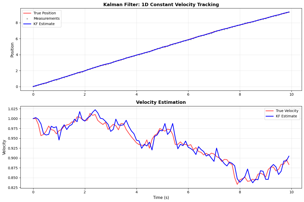
Example: 1D Constant Velocity Tracking
Finally, show an example of your algorithm in action.This should be a simple example that gets the idea across on how to use your algorithm in a standard simulation loop.
We track a target moving in 1D with (approximately) constant velocity, where we only observe its position. We suppose this is a linear system with zero-mean Gaussian process and measurement noise.
Note that even though we only measure position, the Kalman filter is able to estimate both position and velocity. This is because the filter uses the system’s dynamical model (constant velocity motion) to infer velocity from the sequence of position measurements. This demonstrates the power of model-based state estimation: by leveraging knowledge of how the system evolves, the Kalman filter can estimate hidden states that are not directly observed.

The diagram above shows the structure of our example: the Target block represents the system being tracked (with 2D state \(x_k = [p_k, v_k]^\top\)), and the Kalman Filter block estimates this state from noisy position measurements \(y_k\). The KF maintains its own state \(z_k = (\hat{x}_k, P_k)\) consisting of the state estimate and covariance.
def target_f(xk, Ak):
    """
    Noise-free state evolution of target.

    Parameters:
        xk: State vector [position, velocity] as column vector, shape (2, 1)
        Ak: State transition matrix for constant velocity model, shape (2, 2)
            Ak = [[1, dt],
                  [0,  1]]

    Returns:
        xk_next: Next state [position, velocity] as column vector, shape (2, 1)
    """
    xk_next = Ak @ xk
    return xk_next


def target_h(xk, Ck):
    """
    Noise-free measurement of target.

    Parameters:
        xk: State vector [position, velocity] as column vector, shape (2, 1)
        Ck: Measurement matrix that extracts position only, shape (1, 2)
            Ck = [[1, 0]]  (measures position, ignores velocity)

    Returns:
        yk: Measurement (position only) as column vector, shape (1, 1)
    """
    yk = Ck @ xk
    return yk


target_block = DynamicalSystem(f=target_f, h=target_h)

kf_block = DynamicalSystem(f=f, h=h)  # f and h are defined above
import numpy as np

rng = np.random.default_rng()

### SIMULATION TIME ############
dt = 0.1
sim_time = np.arange(0, 10, dt)

#### EXPLICIT PARAMETERS #########################

xk = np.array([[0.0], [1.0]])  # initial target state (column vector, pos and vel)

Pk = np.array([[1e-3, 0], [0, 1e-3]])
zk = [xk, Pk]  # initial kf state

# target dynamics and measurment matrices
Ak = np.array([[1, dt], [0, 1]])
Ck = np.array([[1, 0]])


#### IMPLICIT PARAMETERS #########################

Qk = np.array([[1e-4, 0], [0, 1e-4]])
Rk = np.array([[1e-3]])
kf_constant_params = {
    "f": target_block.f,
    "h": target_block.h,
    "Qk": Qk,
    "Rk": Rk,
    "Fk": Ak,
    "Hk": Ck,
}

### HISTORIES #################

true_states = []
measurements = []
kf_state_estimates = []

### SIMULATION ###################################################
for tk in sim_time:

    # Noise-free state evolution
    xk_next, yk = target_block.step(params={"xk": xk, "Ak": Ak, "Ck": Ck})

    # Apply process noise and measurement noise
    process_noise = rng.multivariate_normal(mean=np.zeros(Qk.shape[0]), cov=Qk).reshape(
        -1, 1
    )
    measurement_noise = rng.multivariate_normal(
        mean=np.zeros(Rk.shape[0]), cov=Rk
    ).reshape(-1, 1)

    xk_next = xk_next + process_noise
    yk = yk + measurement_noise

    zk_next, xhatk = kf_block.step(
        params={
            "zk": zk,
            "yk": yk,
            "f_h_params": {"xk": xk, "Ak": Ak, "Ck": Ck},
            **kf_constant_params,
        }
    )

    true_states.append(xk.flatten())
    measurements.append(yk.flatten())
    kf_state_estimates.append(xhatk.flatten())

    xk = xk_next
    zk = zk_next

# Convert to arrays for plotting
true_states = np.array(true_states)
measurements = np.array(measurements)
kf_state_estimates = np.array(kf_state_estimates)
Notes on Usage
What should users of your algorithm know if they want to use it? Add links to outside resources if relevant.
The Kalman filter is an optimal unbiased estimator when all of the following conditions hold:
Linear dynamics: The system evolution and measurement models are linear (or have been linearized)
Gaussian noise: Process noise and measurement noise are approximately Gaussian
Known covariances: The noise covariance matrices \(Q\) and \(R\) can be estimated or characterized
If your system is nonlinear, consider using the Extended Kalman Filter (EKF) or Unscented Kalman Filter (UKF) instead. If your noise is non-Gaussian (e.g., heavy-tailed, multimodal), consider particle filters or other robust estimators.
Jacobian Requirements
For linear systems, the Jacobians are simply the system matrices:
State transition Jacobian: \(F_k\) is the linearized dynamics matrix
Measurement Jacobian: \(H_k\) is the linearized measurement matrix
In this implementation:
Fkshould be the Jacobian \(\frac{\partial f}{\partial x}\) evaluated at the current estimateHkshould be the Jacobian \(\frac{\partial h}{\partial x}\) evaluated at the current estimate
For time-invariant linear systems (constant matrices), these are the same at every time step. For time-varying or nonlinear systems, recompute the Jacobians at each step.
Tuning Guidance
The performance of the Kalman filter depends critically on the noise covariance matrices:
Process noise \(Q\): Larger values → filter trusts model less, adapts faster to changes
Measurement noise \(R\): Larger values → filter trusts measurements less, smoother estimates
Initial covariance \(P_0\): Set based on initial uncertainty. Large values indicate high initial uncertainty; the filter will converge as measurements arrive.
For practical tuning, see this guide on tuning Kalman filters.